Graph Data Structure

To represent graphs that should be laid out, the Eclipse Layout Kernel provides a robust EMF-based data structure. This page is about describing that graph data structure.

Terminology

Graphs

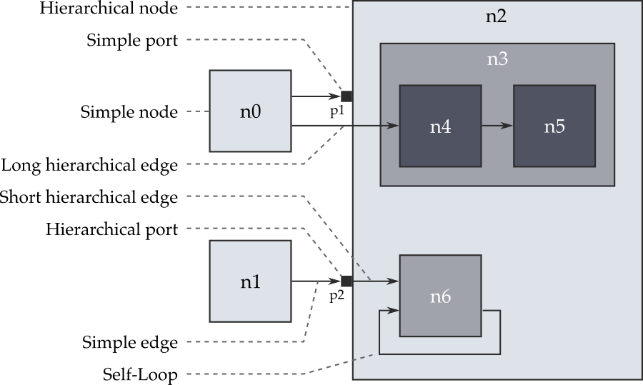
This is a simple example graph along with the terminology that goes with it.

Inclusion Trees

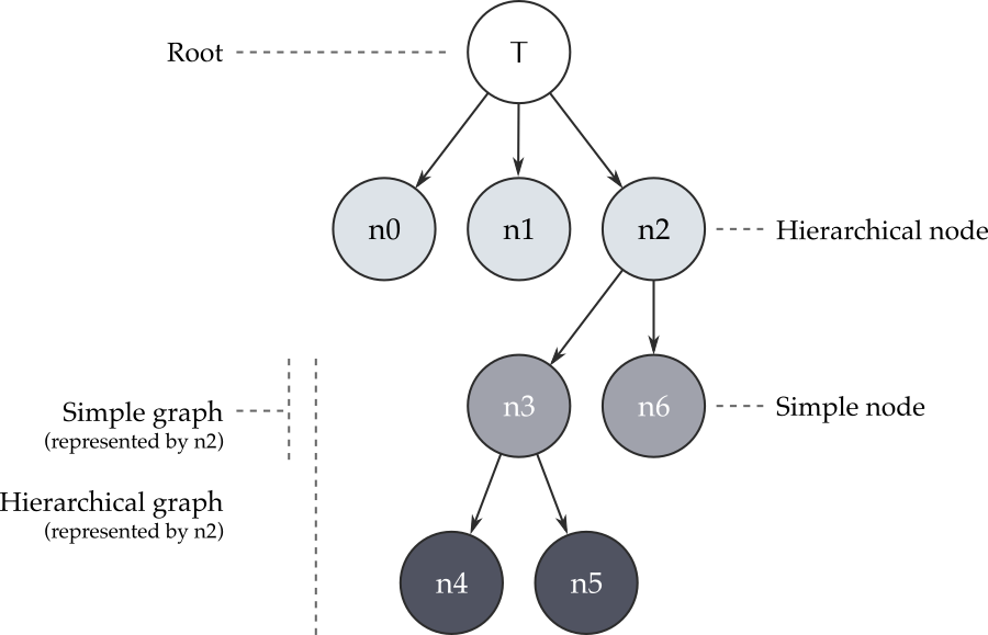
Inclusion trees capture the hierarchical structure of a graph. See below for the inclusion tree of the graph we just saw, along with the terminology that goes with it.

Definitions

• Inclusion Tree: The parent-child relationships of all nodes. This is basically the node containments in the EMF data structure. Note that in an ELK graph, the tree always has a single root node that represents the drawing area. Top-level nodes are children of that root node.

• Graph: A set of nodes and edges and whatever else belongs to them (labels, ports, …).

  • Simple Graph: All children of a single node. The node represents that simple graph. This means that if the objects that the graph consists of are to be passed to a layout algorithm, this is done by simply passing the node object that represents that graph.

  • Hierarchical Graph: All descendants of a single node. Although the word “all” is a bit too strong here: we may choose to exclude all descendants of one of the node’s descendants. Similar to simple graphs, that single node represents the hierarchical graph. The root node represents the whole graph (see below) and is simply a special case of this rule.

• Node:

  • Simple Node: A node that does not contain child nodes.

  • Hierarchical Node: A node that contains child nodes.

• Edge:

  • Simple Edge: An edge that connects two nodes in the same simple graph. This of course implies that the edge’s source and target nodes both have the same parent node.

  • Hierarchical Edge: An edge that is not simple.

    • Short Hierarchical Edge: A hierarchical edge that only has to leave (or enter) a single hierarchical node to get to its target. Thus, a short hierarchical edge connects nodes in adjacent layers of hierarchy.

    • Long Hierarchical Edge: A hierarchical edge that is not a short hierarchical edge.

• Port: An explicit connection point on a node for edges to connect to.

  • Simple Port: A port on a simple node, or a port that does not have incident hierarchical edges.

  • Hierarchical Port: A port on a hierarchical node that has incident hierarchical edges.

• Root Node: The root of the inclusion tree.

  • Root Node of a Graph: The lowest common ancestor of all nodes in the graph.

Graph Data Structure

The Meta Model

The ELK Graph meta modelh looks like this:

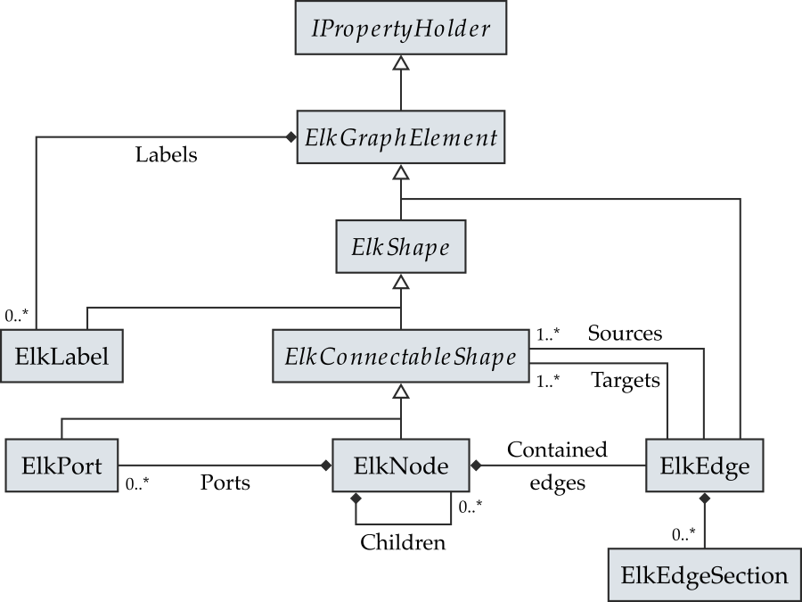
It contains the following types:

• IPropertyHolder

  Instances of this type hold a map of properties to values. The usual use case is for clients to set properties on elements that influence the behavior of layout algorithms, but nothing stops layout algorithms from using properties internally as well. Properties are so important, in fact, that they have their own page of documentation.

• ElkGraphElement

  Everything in an ELK graph is an ElkGraphElement. All graph elements hold properties and a list of labels.

• ElkShape

  The supertype of every kind of graph element that can be described by a rectangular area: nodes, ports, and labels. Shapes have an x and y coordinate as well as a width and a height.

• ElkLabel

  Labels are used to represent text in a diagram and can be attached to all other elements, including other labels. Although we currently have no layout algorithm that supports labeled labels. Each label has the text it should display as a property.

• ElkConnectableShape

  Edges can connect to ports that belong to nodes or directly to nodes. Both are connectable shapes, which can act as the sources or targets of edges. The ElkGraphUtil class contains methods to turn a connectable shape into the corresponding port (if any) or node.

• ElkPort

  Ports represent explicit attachment points provided by nodes. Each port belongs to exactly one node.

• ElkNode

  Nodes could be considered the primary ingredient of an ELK graph. They can contain child nodes, which is why the graph itself is represented by an ElkNode as well (instead of introducing an additional ElkGraph class). Nodes can contain ports that edges can connect to. They also contain a list of edges. These edges are not the ones that connect to a node itself, but are the edges that connect its children. The reason for this is that EMF, the technology behind the ELK graph, requires every model element to be contained in another, which influences how a graph is serialized. Clients that build ELK graphs using the methods in ElkGraphUtil usually need not worry about this.

• ElkEdge

  An edge connects at least one source to at least one target, implying that they are always directed and can be hyperedges (multiplie sources or targets). The path an edge takes through a diagram is described by its list of ElkEdgeSection instances.

• ElkEdgeSection

  Describes part of the path an edge takes through a diagram. First and foremost, each edge section has a single parent edge. Routing-wise, it has x and y coordinates for its start and end points and a possibly empty list of bend points. Edges that connect only one source to one target have a single edge section. Hyperedges will have more. To be able to structure them properly, an edge section has a beginning and an end. Both can be either a connectable shape (if the section is an outer section of the edge) or another edge section.

Working With the Graph Data Structure

Since ELK graphs are based on EMF, you can simply obtain an instance of the ElkGraphFactory interface and start creating graph elements. To make things easier, however, the ElkGraphUtil contains a number of utility methods in different categories:

• Graph Creation: There are a number of methods whose names begin with create that can be used to create and initialize graph elements. For instance, the createSimpleEdge(source, target) method not only creates an ElkEdge, but also sets its source and target and, as a bonus, adds it to the list of contained edges of the correct node, all in a single method call.

  One method of particular value to layout algorithm developers is firstEdgeSection(edge, reset, removeOthers), which returns the first edge section of the given edge, optionally resetting its layout data and removing all other edge sections. If the edge doesn’t have any edge sections yet, one is created and added to it. This method is handy for applying layout results.

• Edge Containment: Unless one uses one of the create methods to create edges, finding the node an edge should be contained in may be annoying (thus, don’t). The updateContainment(ElkEdge) method automatically computes the best containment and puts the edge there. This requires at least one of the edge’s end points to be set, since that is what determines the best containment.

  While computing the containment is a little intricate (hence the utility method), the actual rule that determines the best containment is rather simple: it is the lowest common ancestor of all end points, where the ancestors of a node are defined as the sequence of nodes from the node itself to the graph’s root node. Taking the graph at the top of this page as an example, the rule has the following implications for different types of edges:

  1. The simple edge that connects n4 to n5 is contained in n3 since that is the lowest common ancestor of both nodes.

  2. The short hierarchical edge that connects n2 to n6 is contained in n2 since n2 is its first ancestor.

  3. The long hierarchical edge that connects n0 to n4 is contained in the node that represents the whole graph (the root node), since that is the first common ancestor of n0 and n4.

  The self loop that connects n6 to itself might be considered an exception to this rule. It is not contained in n6, but in n2, since it runs through the simple graph represented by n2. This is true even if the self loop is routed through the insides of n6, which layout algorithms may or may not support.

• Convenience Methods: There are a number of convenience methods, for example to iterate over all of a node’s incoming or outgoing edges, to find the node that represents the simple graph an element is part of, and more.