Re: [sumo-user] The mesoscopic model

[Jakob Erdmann <namdre.sumo@xxxxxxxxx>]

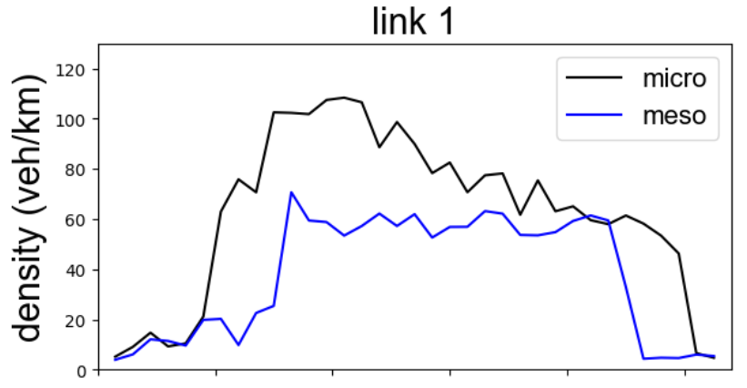
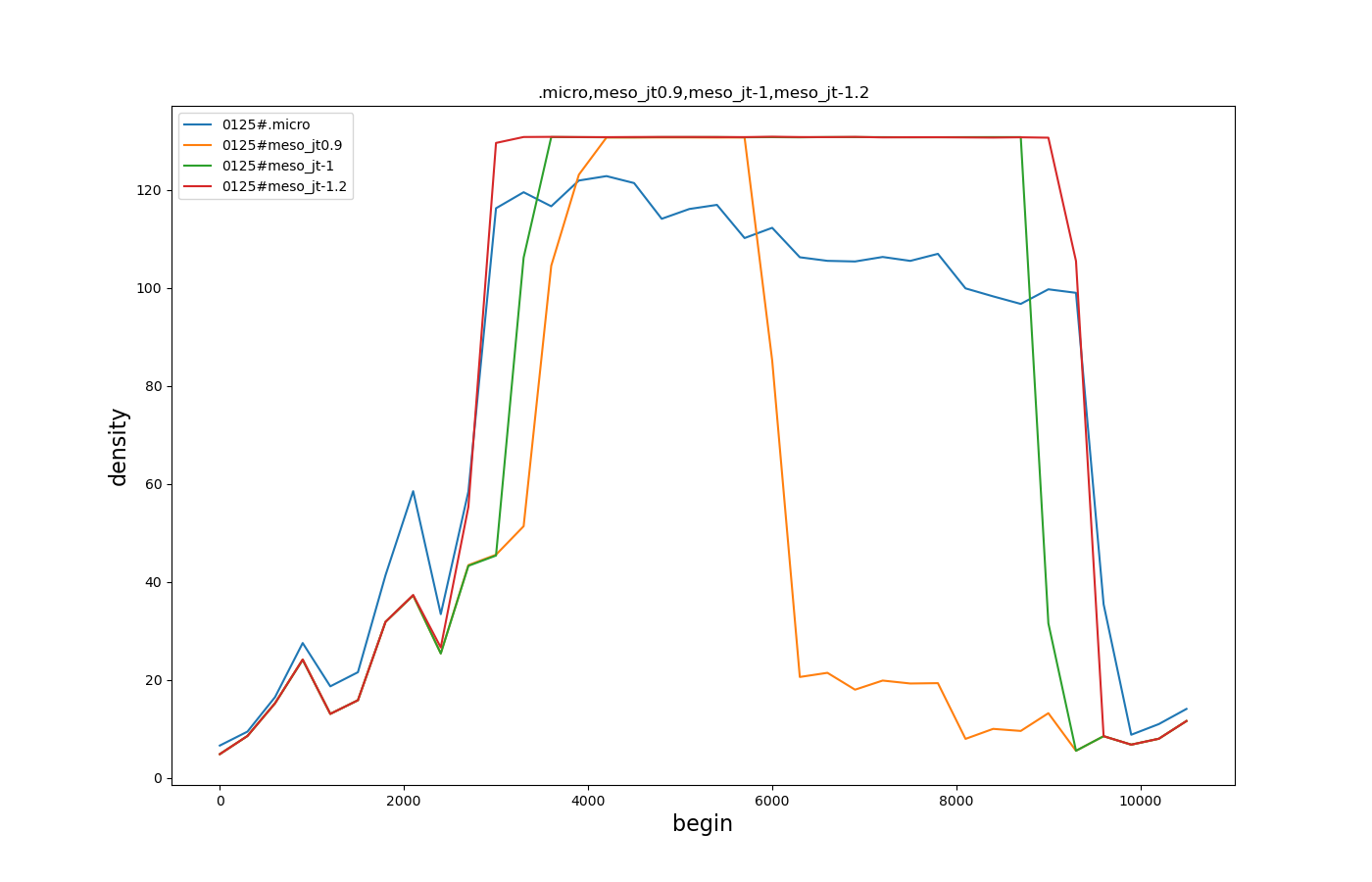
My graph was obtained by running the provided simulation files with the modified --meso-jam-threshold and then plotting with:

sumo/tools/visualization/plotXMLAttributes.py --legend --filter-ids 0125 -x begin -y density

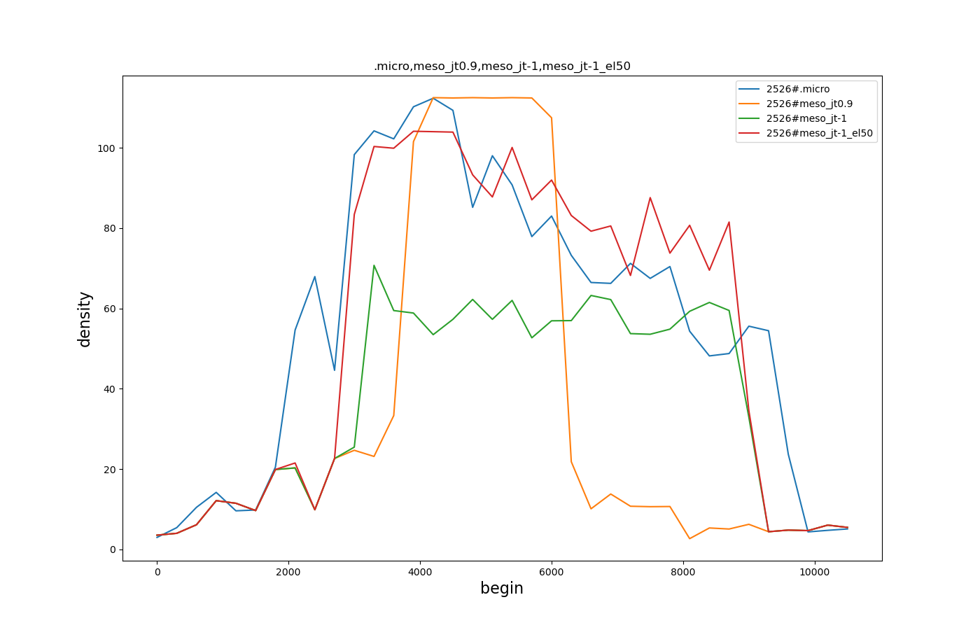
I did not notice that there was still a significant discrepancy between meso and micro densities for the second link (2526) even with --jam-threshold -1 and discovered the following:

The jam is created by having an additional inflow from side road 3328 and in your setup this inflow is underestimated in meso for the following reason:

- in micro, the distribution of traffic is shown to be inhomogenic: there is a queue at the red light but the rear of the lane is free

- in meso jam state is always considered for a full segment and your intersection spacing is so close that each edge only has a single segment. This means once a the queue is sufficiently long, inflow from the side is computed in jam-jam mode with much reduced flow

- by setting option meso-edgelength 50 the difference between meso and micro mostly goes away (see plot below). This is, because this option creates two segments with an individual jam state on every edge and thereby allows inflow from the side in jam-free mode.

> The flat density in the jam state indeed means that the propagating space is actually not considered.

No, the flat density comes about because inflow and outflow are in balance (flow rate is dominated by the traffic light) and the low level was explained above by insufficient inflow from the side road

> Then the remaining question I would like to ask is that whether the definition of this jam threshold occupancy is the same as the logic of the critical density on a fundamental diagram.

Yes. By model definition, the flow on a segment starts to degrade once this density is exceeded. 

Please note that sumo-gui gives misleading threshold values for your network due to the presence of forbidden lanes (https://github.com/eclipse-sumo/sumo/issues/16449)

regards,

Jakob

Am Mi., 2. Apr. 2025 um 18:09 Uhr schrieb Ni Ying-Chuan <ying-chuan.ni@xxxxxxxxxxxxxxxx>:

Dear Jakob and SUMO team,

 

Thank you very much for the answer.

Yes, I see the influence of the jam threshold value now although in my simulation the density evolution after changing it to -1 (see below) is quite different from the plot you showed me.

The flat density in the jam state indeed means that the propagating space is actually not considered.

Then the remaining question I would like to ask is that whether the definition of this jam threshold occupancy is the same as the logic of the critical density on a fundamental diagram.

Thanks a lot!

 

Best regards,

Ying-Chuan

 

From: Jakob Erdmann <namdre.sumo@xxxxxxxxx>
Sent: Wednesday, April 2, 2025 5:21 PM
To: Sumo project User discussions <sumo-user@xxxxxxxxxxx>
Cc: Ni Ying-Chuan <ying-chuan.ni@xxxxxxxxxxxxxxxx>
Subject: Re: [sumo-user] The mesoscopic model

 

Hello,

Your concern may be valid insofar the current algorithm possibly overestimates void space propagation (especially on short edges).

However, the mismatch between microscopic and mesoscopic behavior is mainly caused by an unfortunate choice of the parameter meso-jam-threshold 0.9

With this setting, the meso model almost never enters the jammed state.

The default values from Eissfeldts dissertation was set to 0.29 (calibrated for motorways). This is unsuitable for road networks with a wide range of speed limits.

For this reason the default value of -1 is used to compute a dynamic threshold for each edge (see https://sumo.dlr.de/docs/Simulation/Meso.html#meso-jam-threshold).

The default works much better than 0.9 and an even better fit is reached with -1.2

For clarity, the plot only shows the most upstream edge which also showed the highest discrepancy.

 

Note, that the lower maximum density in sumo is an artifact of the insertion rules: there are no half cars and in micro, the next car can only enter if a full gap has traveled to the start of the edge. In contrast, meso cars are inserted as soon as the total space on an edge permits it.

 

regards,

Jakob

 

Am Mi., 2. Apr. 2025 um 10:27 Uhr schrieb Ni Ying-Chuan via sumo-user <sumo-user@xxxxxxxxxxx>:

Dear SUMO team,

 

I would like to test the accuracy of the mesoscopic model in SUMO, which is based on the Eissfeldt's dissertation (2004).

The model describes that when there is a spillback (the downstream edge is completely occupied), the headway from upstream edge to the downstream edge is the time required for a space to travel upstream, which is of course theoretically correct.

However, in the case I implemented, it seems that the headway is immediately updated in the following time steps when a vehicle leaves the downstream link (the link becomes free because of the smaller number of vehicles), while the void space hasn't yet arrived at the upstream end actually.

The resulting link density evolutions are hence very different from the microsimulation ground-truth. The congestion ends earlier because spillback is not properly considered.

Attached are the case study of a simple urban corridor.

 

Could you let me know if this is a problem that was overlooked? Or is there any parameter I need to change to make the meso-simulation better?

If it indeed is a problem, I can share a solution. Please feel free to contact me via the email below to discuss.

Thank you very much. I look forward to your reply.

 

Kind regards,

Ying-Chuan Ni

 

--------------------------------

Email: ying-chuan.ni@xxxxxxxxxxxxxxxx

Traffic Engineering Group (SVT)

Institute for Transport Planning and Systems (IVT)

ETH Zurich

 

 

_______________________________________________
sumo-user mailing list
sumo-user@xxxxxxxxxxx
To unsubscribe from this list, visit https://www.eclipse.org/mailman/listinfo/sumo-user