This document explains the domain of the Logistics, Specification and Analysis Tool (Eclipse LSAT™), provides explanation to the underlying architecture of Eclipse LSAT™, and presents the workflows for different analysis techniques included in Eclipse LSAT™. This document is intended to assist stakeholders involved in the software development of Eclipse LSAT™, whether new or old, to understand the existing architecture of Eclipse LSAT™.
-
Section 1 is an introduction to Eclipse LSAT™ and its different performance analysis techniques.
-
Section 2 describes the architecture of Eclipse LSAT™.
-
Section 3 describes related workflows.
-
Section 4 gives an overview about different plugins in Eclipse LSAT™.
-
Section 5 provides information on development for Eclipse LSAT™.
-
Appendix A provides information on how to add your own custom motion profile to Eclipse LSAT.
-
Appendix B provides information on how to implement a custom motion calculator with Json.
| A PDF version of this document is also available. |
1. Introduction
1.1. Scope
Eclipse LSAT™ allows convenient modeling mechanism for physical machines. In addition to modeling of logistics, the following analysis techniques are also included in Eclipse LSAT™.
-
Automatic generation of optimal logistics in terms of makespan/throughput.
-
Visualization of logistics in the form of Gantt charts.
-
Conformance checking of traces against a specification.
Thus, Eclipse LSAT™ offers design-space exploration for the physical machine which enables engineers to predict performance at a design time.
1.2. Tools
The following tools are used for designing architecture and modeling environment of Eclipse LSAT™.
-
Eclipse Modelling Framework (EMF) (https://www.eclipse.org/modeling/emf/)
-
QVTo (https://projects.eclipse.org/projects/modeling.mmt.qvt-oml)
-
Xtend (https://www.eclipse.org/xtend/)
-
Xtext (https://www.eclipse.org/Xtext/)
-
Sirius (https://www.eclipse.org/sirius/)
-
Eclipse Layout Kernel (https://www.eclipse.org/elk/)
The following tools are used for performance analysis.
-
Eclipse ESCET (Supervisory Control Engineering Toolkit) (https://www.eclipse.org/escet)
-
Eclipse TRACE4CPS (https://www.eclipse.org/trace4cps)
2. Architecture
This section presents the architecture used to design and analyze logistics in Eclipse LSAT™. In the first subsection, we explain the domain languages of Eclipse LSAT™. In addition to domain languages, we also have analysis languages to perform performance analyses which are explained in the second subsection.
2.1. Domain Languages
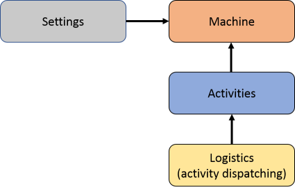
Logistics in Eclipse LSAT™ are modeled by separating different concerns in a modular way, as shown in the following figure. Typically, persistence of each domain language is implemented in Xtext. For graphical editing, Sirius representation is implemented.
2.1.1. Machine
This module describes the plant in terms of resources and peripherals with their capabilities and restrictions. For example, machine corresponds to the plant or a part of the plant. Similarly robot and its clamp correspond to resource and peripheral respectively. Thus, we describe the plant on a logical level using the machine module.
We express motion in robots by using symbolic coordinates and physical coordinates to decouple physical implementation from logical specification. For example, for representing symbolic coordinates, the cylindrical coordinate system is used. Whereas, the angular coordinate system is used to represent physical coordinates. The cylindrical system is shown in the figure below.

The cylindrical coordinate system contains origin O, polar axis A, and longitudinal axis L. The dot is a point with radial distance ρ ( R ), angular coordinate φ (Phi), and height z.
A robot in angular coordinate system is shown in the figure below. In this figure, the robot is present at the cylindrical coordinate with angular coordinates ϴ1 (Th1) and ϴ2 (Th2) and height z.

The angular coordinates can be calculated from cylindrical coordinates as follows.
Th1 = Phi - acos((R - E)/2/L)
Th2 = Phi + acos((R - E)/2/L)
Machine Metamodel
The machine metamodel is shown in the figure below. Within industrial context, a machine model instance typically represents a physical machine.

Machine is the root of a model. It contains resources, peripheralTypes and imports. Resource corresponds to resources in a machine, e.g., a robot. A resource optionally contains resource items when there are multiple instances of the same resource available. Each resource contains peripherals, e.g., clamp of a robot. Each peripheral refers to PeripheralType that corresponds to the type of the peripheral, e.g., linear motor is of a type motor.
Each peripheral type defines the action a peripheral can perform using ActionType. These actions are typically called 'simple actions', which are defined as actions which are atomically executed and consumes a particular amount of time.
Motion specified between positions
As mentioned in Machine, motion in robots can be defined in symbolic coordinate system and physical coordinate system. The physical coordinate system is modeled by setPoints. Similarly, the symbolic coordinate system is modeled by axes. Axes and setpoints contain units represented by Unit. If the unit of an axis differs from the unit of its set points, conversion in PeripheralType converts a symbolic location in the symbolic coordinate system to a physical location in the physical coordinate system.
The positions a peripheral can take in the symbolic coordinate system is represented by SymbolicPosition contained in Peripheral. The allowed moves by a peripheral between symbolic positions are represented by Path. Paths can be of three types as follows.
-
UnidirectionalPath corresponds to a path with only one direction.
-
BidirectionalPath corresponds to a bidirectional path.
-
FullMeshPath corresponds to a path where all moves from a location to another location are allowed.
For example, if a peripheral have symbolic position pos1 and pos2, and there is a unidirectional path between them, then the peripheral can only move from pos1 to pos2, but not in the opposite direction.
The speed profile for the paths is represented by Profile. The source or targets of paths is specified by PathTargetReference that refers to a symbolic position. settling defines the settling axes on paths.
For all axes of a movable peripheral, we have to define positions. For example, in the following figure, we can see positions for X and Y axes.


To define positions for an axis, we define a key-value pair AxisPositionsMapEntry in the machine metamodel, where key is an axis and values are positions (similar to AxisPositionsMapEntry).
The machine metamodel contains some operations, as explained in the following.
| Name | Class | Description |
|---|---|---|
getPosition(axis Axis) |
SymbolicPosition |
Returns position of the axis for this specific symbolic position. |
getOutgoingPaths() |
SymbolicPosition |
Returns the list of outgoing paths from a symbolic position. |
getSources() |
Path |
Returns the source of a path. |
getTargets() |
Path |
Returns the target of a path. |
Motion specified as distances
Instead of positions, distances can be specified. Distances only describe a move of a certain distance where the location is unknown or not relevant. Typically used for circular, belt or mill movements. Either (AxisPositions,SymbolicPositions,Paths) or Distances must be specified. They are mutual exclusive.

2.1.2. Settings
This module provides physical settings for the machine. For example, for peripherals, we can specify the settings for physical locations and speed profiles.
Separating settings specification from machine specification allows us to have design-space exploration by analyzing the same machine for different physical settings.
Settings Metamodel
The settings metamodel is shown in the figure below. Using the setting metamodel, we can specify the physical settings for the Twinscan machine.
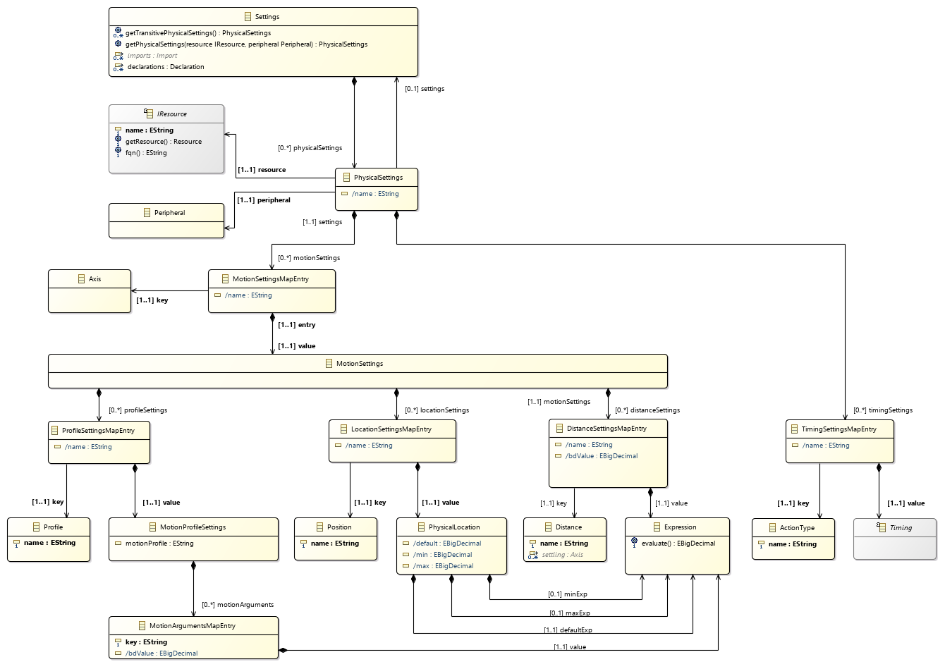
Settings is the root of a model. It contains PhysicalSettings and Import. PhysicalSettings contains settings associated to a peripheral of a resource, and Import imports machine files containing the resources. In PhysicalSettings, we can,
-
set timing information for an action,
-
assign movement related parameters, i.e., motion parameters for a motion profile per axis,
-
allocate physical locations to symbolic positions per axis.
-
allocate physical distances to symbolic distances per axis.
For (1), PhysicalSettings contains TimingSettingsMapEntry. It is a key-value pair, where key is a ActionType, and value is Timing. Thus, we can assign timing for each action.
For (2), (3) and (4), PhysicalSettings contains MotionSettingsMapEntry, which is again a key-value pair. As (2), (3) and (4) are assigned for each axis, the key is Axis. The value is MotionSettings.
For (2), MotionSettings contains ProfileSettingsMapEntry, which is also a key-value pair. As we specify the movement related parameters per speed profile, the key is Profile. The value is MotionProfileSettings that defines the motion profile to use and contains a MotionArgumentsMapEntry, which is again a key-value pair of which the key is the motion profile parameter and the value is an Expression that defines the argument value.
For (3), MotionSettings contains LocationSettingsMapEntry, which is also a key-value pair. The key is Position and the value is an Expression that defines the physical location.
For (4), MotionSettings contains DistanceSettingsMapEntry, which is also a key-value pair. The key is Distance and the value is an Expression that defines the physical distance.
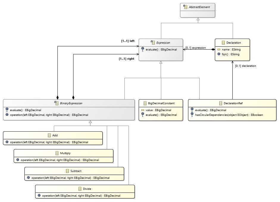
Expressions Metamodel
Expression is the interface to all expression types. Expression.evaluate() returns the evaluated result of the expression as BigDecimal
Supported expressions are:
-
BinaryExpressions : Add, Multiply, Subtract and Divide.
-
DeclarationRef: A Reference to a Declaration.
-
BigDecimalConstant: a constant value.
Expressions are used in Settings and Timing MetaModel
| TODO: describe timing metamodels |

2.1.3. Activities
Activity diagrams are graphical representations of workflows of stepwise activities and actions with support for choice, iteration and concurrency (see https://en.wikipedia.org/wiki/Activity_diagram). In the context of Eclipse LSAT™, the Activities module composes high level actions that a resource can perform into activities. For example, let us assume a robot capable of performing two actions A1 and A2. The action A1 specifies moving of the robot towards the pre-aligner (PA) position and the action A2 specifies clamping of a product by the robot. We can compose these actions into an activity toPAandClamp in which the action A1 is executed before the action A2.
It is also worth mentioning that Eclipse LSAT™ does not support all Activity diagram functions, e.g., iteration and choice.
Activity Metamodel
The activity metamodel is shown in the following figure. Using the activity metamodel, we can model actions that a resource can perform.
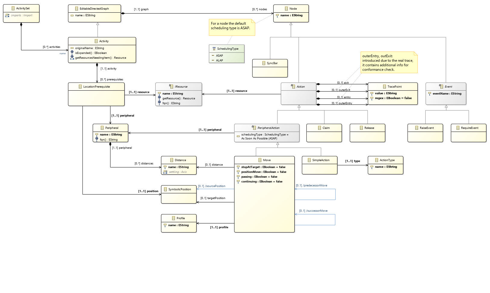
ActivitySet is the root of a model. It contains Activity and Import. Activity represents the activities containing the actions a peripheral can perform. As activities have, in essence, a directed graph structure, Activity is a type of EditableDirectedGraph (see EditableDirectedGraph Metamodel).
EditableDirectedGraph contains Node representing the nodes in a graph. Node has three subtypes, i.e., SyncBar, Action and Event. Actions represents actions, syncbars are used to specify synchronization between actions and events can be used to specify synchronization across activities. Action contains TracePoint that is used for conformance checking of traces (see Conformance Checking subsection). As action is defined for a resource, Action has an association with Resource.
Action has three subtypes, explain as follows.
-
Claim represents the claiming of a resource. Typically, claim is the start action in the activity diagram in which a resource is claimed and rest of the actions take place afterwards. In typical activity diagram workflows, the start action is shown as a black circle.
-
Release represents the releasing of a resource. Typically, release is the final action in the activity diagram in which a resource is release after rest of the actions have taken place. In typical activity diagram workflows, the final action is shown as a encircled black circle.
-
PeripheralAction represents the actions involving a peripheral. For example, clamping of a product by the peripheral clamp of a robot. Therefore, PeripheralAction has an association with Peripheral.
PeripheralAction are of two types, as explained in the following.
-
SimpleAction represents simple actions like clamping or unclamping of a robot hand.
-
Move represents the actions involving movements between symbolic positions or over distances. Move has a boolean attribute stopAtTarget. If this attribute is true, then the peripheral does not perform any further movement and the current movement ends in stand-still. If this attribute is false, then another movement follows the current movement.
Activity also contains LocationPrerequisite that represents the initial location for all peripherals that move between positions for an activity.
2.1.4. Logistics
This module schedules activities specified in the activity module. For example, if we have two activities toPAandClamp and Measure, we can schedule these activities in such a way that the activity toPAandClamp is executed before the activity Measure.
Thus, we use the logistics module to specify the timing and throughput requirements.
Logistics Metamodel
The logistics metamodel is shown in the following figure. This metamodel is used to schedule activities modeled using Activity Metamodel.

ActivityDispatching is the root of a model. It contains DispatchGroup, ResourceIterationsMapEntry and Import.
DispatchGroup:
-
represents a group of activity dispatches.
-
has an attribute offset that represents the offset time before the activities to start.
-
has an attribute yield that describes the number of products one Repeat yields.
-
has an attribute iteratorName that describes the name of the item that is dispatched. The default is 'iteration'.
-
contains one or more Dispatch that represents dispatching of an activity. Therefore, Dispatch has an association with Activity.
-
contains a list of Repeats.
Repeat describes how often the activities in a DispatchGroup must be repeated. For flexible range support (similar to how pages are specified in a print command) Repeat contains a range (start, count, end, numberRepeats). To support multiple ranges multiple Repeats can be used in a DispatchGroup.
ResourceIterationsMapEntry is used to identify where the specification can be optimized for throughput performance of the system. ResourceIterationsMapEntry is also used to show an overview of the throughput per resource and the throughput of the total activity dispatching sequence. Thus, ResourceIterationsMapEntry is a key-value pair, where key is Resource representing the resource for which the throughput is calculated, and value is EIntegerObject representing the number of iterations.
HasUserAttributes supports a list of key-value pairs that can be added to a DispatchGroup or Dispatch. This way user specific metadata can be added to the model.
2.2. Analysis Languages
2.2.1. DirectedGraph Metamodel
The DirectedGraph metamodel is shown in the following figure.

DirectedGraph is the root of a model. It contains Node and Edge. Node represents nodes in a graph and Edge represents edges in a graph. Each node has outgoingEdges and incomingEdges. Similarly, each edge has one sourceNode and targetNode.
For stochastic analysis in Eclipse LSAT™, various stochastic annotations have to be assigned to nodes and edges. This is done using Aspect. Directed graphs can also contain subgraphs represented by subGraphs.
The DirectedGraph metamodel contains an operation, as explained in the following.
| Name | Class | Description |
|---|---|---|
allNodesInTopologicalOrder():Node |
EditableDirectedGraph |
Returns all nodes in a directed graph in a topological order. |
2.2.2. EditableDirectedGraph Metamodel
Activity flow in activity specifications are represented in a textual representation as follows.
A1 → A2 → A3
where A1, A2 and A3 represent activities and arrows represent the flow between activities. We can also see this example in the form of a directed graph where activities are represented by nodes and arrows between activities represent edges. Thus, we can represent this example using DirectedGraph Metamodel.
However, Xtext is based on LL(k) (see https://en.wikipedia.org/wiki/LL_parser), which does not allow left recursive grammar. Thus, we cannot concatenate edges using DirectedGraph Metamodel. It means that if want to use DirectedGraph Metamodel to represent the aforementioned activity flow, we have to write two edges, where the first edge is between A1 and A2, and the second edge is between A2 and A3.
To overcome this challenge, we built another metamodel termed as EditableDirectedGraph metamodel, where the target of the first edge in the aforementioned example is A2 → A3 instead of A2. Similarly, A3 is the target of the second edge. In this way, we can concatenate different edges.
The structure of these directed graphs is captured by the EditableDirectedGraph metamodel. In the following, the EditableDirectedGraph metamodel is described.

EditableDirectedGraph is the root of a model. It contains Node and Edge. To facilitate concatenation of edges in the textual syntax, Edge contains a class EdgeTarget that has a subtype TargetReference. In the textual syntax, target of an edge is represented by target which can refer to edge or node. Thus, target of an edge can be another edge or a node (if it is the last node in the activity flow). For example, in the running example, target of the first edge is the next edge A2 → A3. As A3 is the last node in the activity flow, target of the second edge is A3.
Similarly, outgoingEdges of a node are determined by the association sourceReference.
2.2.3. Scheduler Metamodel
The scheduler metamodel serves as a basis for the scheduling activities workflow (see Scheduling activities including Gantt chart visualization). In the following, the Scheduler metamodel is described.

It consists of five parts as explained in the following.
Dispatch Graph
Dispatch Graph is used to convert activity dispatching sequence to a directed graph. Therefore, DispatchGraph is a type of TaskDependencyGraph that refers to DirectedGraph Metamodel. DispatchGraph has an association to Dispatch that refers to Logistics Metamodel. Dispatch contains DispatchGroup that also refers to Logistics Metamodel. DispatchGroup has an association with DispatchGroupTask that is a type of Task.
ActionTask
Task has also another subtype ActionTask that is used to convert actions in Activity Metamodel to a graph. ActionTask has three subtypes, as explained in the following.
-
ClaimTask represents the task of claiming a resource.
-
Release represents the task of releasing a resource.
-
PeripheralAction represents the actions involving a peripheral.
Resource
In the scheduling activities workflow (see Scheduling activities including Gantt chart visualization), Gantt charts are generated per resources. Therefore, we need to extract related resources from the activity dispatching sequence. To achieve this objective, we have Resource in the scheduler metamodel. Resource has three subtypes, as explained in the following.
-
PeripheralResource represents a Resource whose peripheral has performed an action, e.g., a move or an atomic action.
-
ClaimReleaseResource represents a Resource that is claimed or released.
-
DispatchGroupResource represents a Resource involved in an activity sequence.
ScheduledTask
ScheduledTask represents the scheduled task. It has the following attributes.
-
startTime represents the starting time of a task.
-
endTime represents the finishing time of a task.
-
sequence represents the sequence of scheduled activities to which the task belongs.
ScheduledTask has a subtype ClaimedByScheduledTask that can claim and release a scheduled task.
EventStatusTask
EventStatusTask represent the status of an event.
If a particular event is raised but not consumed yet an 'Outstanding' EventStatusTask is inserted.
If a particular event is waiting but the event is not raised yet an 'Awaiting' EventStatusTask is inserted.
Aspect
As mentioned in DirectedGraph Metamodel, aspects are used to annotate various stochastic features. Therefore, Aspect has a subtype StochasticAnnotation that has an attribute weight representing the timing distribution.
2.2.4. PetriNet Metamodel
A Petri net is a directed graph, in which the nodes represent transitions (i.e. events that may occur, represented by bars) and places (i.e. conditions, represented by circles). The directed arcs describe which places are pre- and/or postconditions for which transitions (signified by arrows).
The PetriNet metamodel is shown in the following figure.

As Petri net can be seen as a type of a directed graph, the root of the PetriNet metamodel is DirectedGraph with a subtype PetriNet. As seen in DirectedGraph Metamodel, DirectedGraph contains Edge and Node. Each edge must contain one source and target node.
As nodes in Petri net represent places and transitions, Edge has two subtypes, i.e., Place and Transition. Initial and final places of a Petri net is represented by initial and final respectively. Places has an attribute token that represents if a place contains a token or not.
The PetriNet metamodel is used for conformance checking of Eclipse LSAT™ activity dispatching traces containing a recorded list of actions against specification. Thus, Place has an association with Action.
To relate a trace to a specification in a better way, we add "trace points" to the activity dispatching specification. In other words, activity dispatching sequence is a set of trace points. Trace points are represented as transitions in our Petri net model. Thus, Transition has an association with TracePoint. Furthermore, sync bars in activity specifications are also represented as transitions in the Petri net model. Therefore, Transition has an association with SyncBar. Lastly, each transition can contain multiple traceLines that provide more information if the conformance checking fails such as line number, time stamp etc. This information is contained as attributes inside TraceLine.
2.2.5. MaxPlus Metamodel
The maxplus metamodel is shown in the figure below.

The maxplus metamodel consists of the following major components.
-
Matrix representing the max-plus matrices.
-
Graph corresponding to the following subtypes.
-
FSM referring to finite state machine used for representing a CIF automata.
-
MPS referring to max-plus state-space.
-
MPA referring to max-plus automaton.
-
As mentioned earlier, there exists two techniques for analyzing performance using max-plus, i.e., max-plus state-space and max-plus automaton. Thus, MPS and MPA are utilized for these techniques respectively.
MaxPlusSpecification is the root of a model. It contains Matrix and Graph. To represents values in matrices conveniently, the maxplus metamodel contains Value that is a data type of double. Matrix contain row vectors which are a subtype of Vector representing that the values contained in the row vectors are of type double. Vector has an attribute values of type Value. The initial value of values is -Infinity.
Graph contains Vertex and Edge. Each vertex can have 0 or more outgoing or incoming edges. Each edge has precisely one source and one target. As explained earlier, Graph has three subtypes as follows.
-
FSM
-
MPS
-
MPA
Vertex has three subtypes as follows.
-
FSMState representing a state in FSM.
-
MPSConfiguration representing a configuration state in MPS.
-
Each MPSConfiguration is associated to exactly one FSMState.
-
-
MPAState representing a state in MPA.
-
Similar to MPSConfiguration, each MPAState has an exactly one association with FSMState.
-
As MPS represents data in the form of columns, each MPSConfiguration contains exactly one ColumnVector. Furthermore, MPAState uses the information in the matrices for performance optimization. For this purpose, MPAState has an association with Matrix, and has the following attributes.
-
matrixRowIndex representing the row index of the matrix.
-
matrixColumnIndex representing the column index of the matrix.
Edge has three subtypes as follows.
-
FSMTransition representing a transition between states in FSM. FSM uses the name of the matrices as labels on the transitions. Thus, FSMTransition has an association with Matrix.
-
MPSTransition representing a transition between states in MPS. MPSTransition has an attribute reward representing the number of products produced by taking this transition. Moreover, MPATransition has another attribute duration representing time involved in taking this transition.
-
MPATransition representing a transition between states in MPA. MPATransition, similar to MPSTransition, has an attribute reward representing the number of products produced by taking this transition. Similarly, MPATransition has also an attribute duration representing time involved in taking this transition.
The maxplus metamodel contains operations, as explained in the following.
| Name | Class | Description |
|---|---|---|
getValue(row EInt, column EInt): Value |
Matrix |
Returns the value at the given row index and column index of a matrix. |
3. Workflows for aspect models
Now, we have explained all metamodels in Eclipse LSAT™. In this section, we describe different analysis techniques available in Eclipse LSAT™ and related workflows.
3.1. Scheduling activities including Gantt chart visualization
This workflow allows us to visualize an activity dispatch sequence in the form of Gantt charts as shown in the figure below.
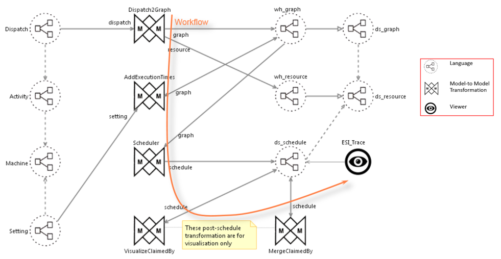
In the following, we explain this workflow.
-
A dispatch model is transformed to a dispatch graph model lsat_graph using a model-to-model transformation Dispatch2Graph written in QVTo. In the dispatch graph model, a resource might be used by multiple activities in the sequence. However, the Dispatch2Graph transformation ensures that only one activity claims a resource at a time. And when the resource is released by the first activity, only then the next active activity can claim that resource. This is done by adding a dependency from the release action of the first activity to the claim action of the second activity. Passive claims (that is claiming a resource to ensure that no actions are performed on the resource) can be done in parallel for multiple activities. (multiple) passive claims are connected to the first preceding active Release. If an active claim is preceded by passive releases than the claim is connected all these passive releases The Dispatch graphs are explained in detail in Scheduler Metamodel.
-
The action execution times of activities in the dispatch model are calculated and added to lsat_graph generated in step 1 using a model-to-model transformation AddExecutionTimes written in Xtend.
-
The lsat_graph model produced in step 2 is transformed to a ds_schedule model using a model-to-model transformation Scheduler written in QVTo. The Scheduler transformation projects the graph on a set of resources in such a way that the the execution times of the nodes are respected. For this purpose, the graph is topologically ordered and scheduled onto the available resources in a asap fashion.
-
The ds_schedule model generated in step 3 is transformed to Eclipse TRACE4CPS using a model-to-text transformation to visualize the ds_schedule model in Eclipse TRACE4CPS.
3.2. Optimal Makespan/Throughput Scheduling
3.2.1. Introduction
The workflow given in the subsection Scheduling activities including Gantt chart visualization explains how we can visualize a activity dispatch sequence. However, if a activity dispatch sequence is written by hand, we cannot guarantee optimality. To overcome this challenge, a workflow which can generate an optimal activity dispatch sequence automatically is added to Eclipse LSAT™.
This workflow is summarized in the figure below.

In this workflow, in addition to Eclipse LSAT™, we also use the following two extra formalisms/tools.
-
Compositional Interchange Format (CIF): CIF is an automata-based modeling language for the specification of discrete event, timed, and hybrid systems. We use CIF to formalize requirements such as life-cycle of products, and synthesize a supervisory controller.
-
Max-Plus Automata: In modeling timed-based systems, quite frequently only the operations max (or min) and + are needed. The max-plus algebra is a mathematical framework that has maximum and addition as the two binary operations. It can be used appropriately to determine marking times within a given Petri net and a vector filled with marking state at the beginning. The MaxPlus metamodel is explained earlier in MaxPlus Metamodel.
3.2.2. Workflow
The figure below shows the workflow used to derive optimal activity dispatching sequence with respect to makespan/throughput.

-
An activity file is transformed to a editable directed graph model lsat_graph using a model-to-model transformation Activity2Graph written in QVTo. The EditableDirectedGraph metamodel is explained earlier in EditableDirectedGraph Metamodel.
-
The action execution times of activities in the dispatch model are calculated and added to lsat_graph generated in step 1 using a model-to-model transformation AddExecutionTimes written in Xtend.
-
The lsat_graph model produced in step 2 along with a CIF file is transformed to a MaxPlus model using a model-to-model transformation Graph2MaxPlus written in QVTo.
-
An algorithm OptimalDispatchGenerator takes as input the MaxPlus model generated in step 3, performs state-space exploration, and outputs optimal activity dispatch sequence OptMaxPlus written in Java.
-
The optimal sequence generated in step 4 OptMaxPlus is transformed to a dispatch file using a model-to-model transformation OptMaxPlus2Dispatch written in Xtend. The model-to-model transformation OptMaxPlus2Dispatch also takes the activity file as an input to determine for which activity, the activity dispatching sequence is generated.
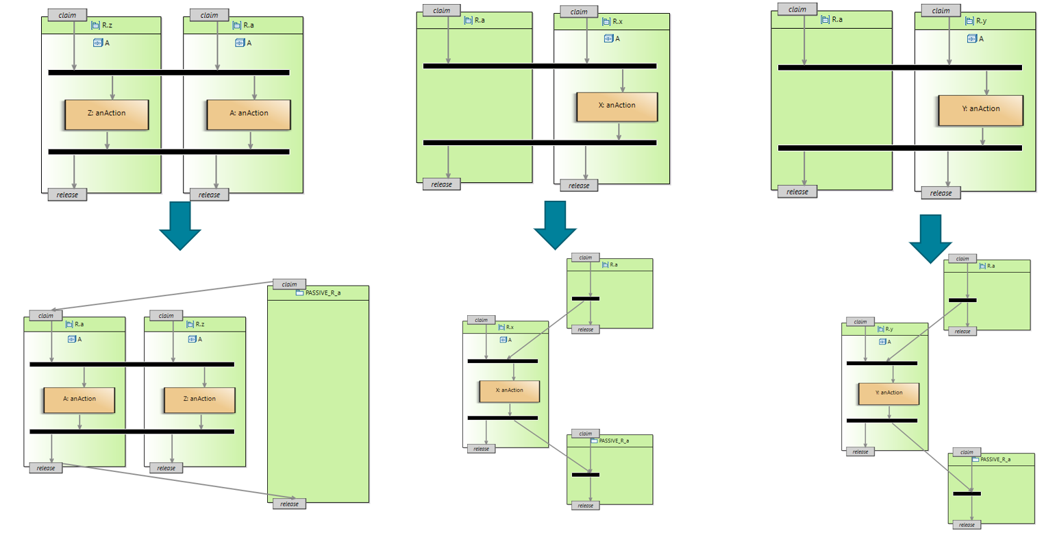
Activity file preprocessing
Before an activity file is transformed via activity2Graph it is made compatible for MaxPlus processing:
-
Events are transformed to Resources with eventName as name. Each event is replaced by a Claim/Release.
-
For Passive claims an extra Resource is introduced with the following conversion rules for a given resource A:
-
If A contains passive claims in any activity then create resource PA.
-
For an activity with actions performed on resource A:
-
claim PA just before claim A
-
release PA just after release A
-
-
For an activity that passively claims resource A
-
release A immediately after claiming A
-
for release replace resource A with resource PA
-
claim PA immediately before releasing it
-
-
Examples:
3.3. Conformance Checking
Eclipse LSAT™ also supports conformance checking of activity dispatching sequence. This is done by first recording a list of actions termed as traces. Second, an activity dispatching sequence is transformed to an equivalent Petri net graph. Last, traces and Petri net graph are fed to the conformance checker, which replays traces on the Petri net to check conformance.
The workflow used to check conformance is shown in the figure below.

-
A dispatching file is transformed to a PetriNets model using a model-to-model transformation dispatch2PetriNets. The PetriNets metamodel is already explained in PetriNet Metamodel.
-
The PetriNets model generated in step 1 is checked for conformance against the Traces files using a model-to-model transformation conformanceCheck written in QVTo.
4. Overview of Plugins
This section presents the overview of plugins in Eclipse LSAT™.
4.1. Machine
| Name | Description |
|---|---|
org.eclipse.lsat.machine.dsl |
Contains the metamodel of machine. |
org.eclipse.lsat.machine.dsl.edit |
Contains generic reusable classes for building editors for EMF models of machine. |
org.eclipse.lsat.machine.teditor |
Contains the Xtext grammar definition of machine and all related components such as parser, lexer, linker. validation, etc. |
org.eclipse.lsat.machine.teditor.ide |
Contains the Xtext language-specific text editor. |
org.eclipse.lsat.machine.teditor.ui |
Contains advanced functionalities such as content assist, outline tree and quick fix. |
org.eclipse.lsat.machine.design |
Contains Sirius modeling projects and representations. |
4.2. Settings
| Name | Description |
|---|---|
org.eclipse.lsat.setting.dsl |
Contains the metamodel of settings. |
org.eclipse.lsat.setting.teditor |
Contains the Xtext grammar definition of settings and all related components such as parser, lexer, linker. validation, etc. |
org.eclipse.lsat.setting.teditor.ide |
Contains the Xtext language-specific text editor. |
org.eclipse.lsat.setting.teditor.ui |
Contains advanced functionalities such as content assist, outline tree and quick fix. |
org.eclipse.lsat.setting.design |
Contains Sirius modeling projects and representations. |
4.3. Activities
| Name | Description |
|---|---|
org.eclipse.lsat.activity.dsl |
Contains the metamodel of activities. |
org.eclipse.lsat.activity.teditor |
Contains the Xtext grammar definition of activities and all related components such as parser, lexer, linker. validation, etc. |
org.eclipse.lsat.activity.teditor.ide |
Contains the Xtext language-specific text editor. |
org.eclipse.lsat.activity.teditor.ui |
Contains advanced functionalities such as content assist, outline tree and quick fix. |
org.eclipse.lsat.activity.diagram.design |
Contains Sirius modeling projects and representations. |
org.eclipse.lsat.activity.diagram.layout |
Contains Eclipse Layout Kernel (ELK) definitions and algorithms. |
4.4. Logistics
| Name | Description |
|---|---|
org.eclipse.lsat.dispatching.dsl |
Contains the metamodel of logistics. |
org.eclipse.lsat.dispatching.teditor |
Contains the Xtext grammar definition of activities and all related components such as parser, lexer, linker. validation, etc. |
org.eclipse.lsat.dispatching.teditor.ide |
Contains the Xtext language-specific text editor. |
org.eclipse.lsat.dispatching.teditor.ui |
Contains advanced functionalities such as content assist, outline tree and quick fix. |
4.5. Directed Graph
| Name | Description |
|---|---|
org.eclipse.lsat.common.graph.directed |
Contains the metamodel of directed graph. |
org.eclipse.lsat.common.graph.directed.editable |
Contains the metamodel of editable directed graph. |
4.6. MaxPlus
| Name | Description |
|---|---|
org.eclipse.lsat.common.mpt.dsl |
Contains the metamodel of maxplus. |
org.eclipse.lsat.common.mpt.dsl.edit |
Contains generic reusable classes for building editors for EMF models of maxplus. |
org.eclipse.lsat.common.mpt.dsl.editor |
Contains a maxplus editor. |
org.eclipse.lsat.mpt.api |
Contains algorithms for computing optimal makespan/throughput. |
org.eclipse.lsat.mpt.feature |
|
org.eclipse.lsat.mpt.ui |
Contains ui features for computing optimal makespan/throughput. |
org.eclipse.lsat.mpt.transformation |
Contains transformations for computing optimal makespan/throughput explained in Section Optimal Makespan/Throughput Scheduling. |
4.7. Scheduling Activities including Gantt Chart Visualization
| Name | Description |
|---|---|
org.eclipse.lsat.scheduler.graph.dsl |
Contains the metamodel of scheduler graph. |
org.eclipse.lsat.scheduler.ui |
Contains ui features for scheduling. |
org.eclipse.lsat.scheduler |
Contains transformations for scheduling explained in Section Scheduling activities including Gantt chart visualization. |
org.eclipse.lsat.scheduler.etf |
Contains transformations from a schedule to Eclipse TRACE4CPS. |
org.eclipse.lsat.motioncalculator.api |
Contains the API for computing timings for different motion types, e.g., point-to-point and distance moves, and motion profiles settings. |
org.eclipse.lsat.motioncalculator.json(.native) |
Contains support classes to easily implement a native motion calculator. |
org.eclipse.lsat.timing |
Contains algorithms for computing timings for different motion types, e.g., point-to-point and distance moves, and motion profiles settings, e.g., normal distribution, triangular distribution, and Pert distribution. |
org.eclipse.lsat.timinganalysis.ui |
Contains ui features for computing timings e.g., playing and exporting animations. |
4.8. Conformance Checking
| Name | Description |
|---|---|
org.eclipse.lsat.petri_net.dsl |
Contains the metamodel of Petri Net. |
org.eclipse.lsat.petri_net.design |
Contains Sirius modeling projects and representations. |
org.eclipse.lsat.conformance |
Contains transformations for conformance checking of traces explained in Section Conformance Checking. |
org.eclipse.lsat.conformance.ui |
Contains ui functions for conformance checking of traces. |
5. Developing
5.1. Development environment setup
Follow these instructions to set up an Eclipse LSAT™ development environment.
To create a development environment (first time only):
-
Get the Eclipse Installer:
-
Go to https://www.eclipse.org/ in a browser.
-
Click on the big Download button at the top right.
-
Download Eclipse Installer, 64 bit edition, using the Download x86_64 button.
-
-
Start the Eclipse Installer that you downloaded.
-
Use the hamburger menu at the top right to switch to advanced mode.
-
For Windows:
-
When asked to keep the installer in a permanent location, choose to do so. Select a directory of your choosing.
-
The Eclipse installer will start automatically in advanced mode, from the new permanent location.
-
-
For Linux:
-
The Eclipse installer will restart in advanced mode.
-
-
Continue with non-first time instructions for setting up a development environment.
To create a development environment:
-
Ensure you are using the latest version of the Eclipse Installer:
-
One option is to download it again, as per the 'first time' instructions above.
-
Another option is to update your existing Eclipse Installer. In the Eclipse Installer, when in advanced mode, click the 'Install available updates' button. This button with the two-arrows icon is located at the bottom-left part of the window, next to the version number. Wait for the update to complete and the Eclipse Installer to restart. If the button is disabled (grey), you are already using the latest version.
-
-
In the first wizard window:
-
Select Eclipse IDE for Eclipse Comitters from the big list at the top.
-
Select 2020-06 for Product Version.
-
For Java 1.8+ VM select a JRE 1.8 that is installed on your local machine. Use the button to the right of the dropdown to manage the installed virtual machines on your system. The JDK can be downloaded from e.g. Oracle or Adoptium.
-
Choose whether you want a P2 bundle pool (recommended).
-
Click Next.
-
-
In the second wizard window:
-
Use the green '+' icon at the top right to add the Oomph setup.
-
For Catalog, choose Eclipse Projects.
-
For Resource URIs, enter
https://gitlab.eclipse.org/eclipse/lsat/lsat/-/raw/develop/lsat.setupand make sure there are no spaces before or after the URL. -
Click OK.
-
-
Check the checkbox for Eclipse LSAT™, from the big list. It is under Eclipse Projects / <User>.
-
At the bottom right, select the develop stream.
-
Click Next.
-
-
In the third wizard window:
-
Enable the Show all variables option to show all options.
-
Choose a Root install folder and Installation folder name. The new development environment will be put at
<root_installation_folder>/<installation_folder_name>. -
Fill in the Eclipse LSAT™ Git clone URL:
-
Committers with write access to the Eclipse LSAT™ official GitLab repository can use the default URL
https://gitlab.eclipse.org/eclipse/lsat/lsat.git. -
Contributors can use the same URL, but as they don’t have write access, they will not be able to push to the remote repository. They can instead make a fork of the official Git repository. Then they can fill in the URL of their clone instead, i.e.
https://gitlab.eclipse.org/<username>/<cloned_repo_name>.git, with<username>replaced by their Eclipse Foundation account username, and<cloned_repo_name>replaced by the name of the cloned repistory, which defaults tolsat.
-
-
For Eclipse Foundation account full name fill in your full name (first and last name) matching the full name in your Eclipse Foundation account. This will be used as name for Git commits.
-
For Eclipse Foundation account email address fill in the email address associated with your Eclipse Foundation account. This will be used as email for Git commits.
-
Click Next.
-
-
In the fourth wizard window:
-
Select Finish.
-
-
Wait for the setup to complete and the development environment to be launched.
-
If asked, accept any licenses and certificates.
-
-
Press Finish in the Eclipse Installer to close the Eclipse Installer.
-
In the new development environment, observe Oomph executing the startup tasks (such as Git clone, importing projects, etc). If this is not automatically shown, click the rotating arrows icon in the status bar (bottom right) of the new development environment.
-
Wait for the startup tasks to finish successfully.
If you don’t open the Oomph dialog, the status bar icon may disappear when the tasks are successfully completed.
If you have any issues during setting up the development environment, consider the following:
-
You can set the following environment variables to force the use of IPv4, in case of any issues accessing/downloading remote files:
_JAVA_OPTIONS=-Djava.net.preferIPv4Stack=true
_JPI_VM_OPTIONS=-Djava.net.preferIPv4Stack=true
After setting them, make sure to fully close the Eclipse Installer and then start it again, for the changes to be picked up.
In your new development environment, consider changing the following settings:
-
For the Package Explorer view:
-
Enable the Link with Editor setting, using the
 icon.
icon. -
Enable showing resources (files/folders) with names starting with a period. Open the View Menu (
 (
( ).
Uncheck the
).
Uncheck the .* resourcesoption and click OK. -
Group projects into working sets.
-
Open the View Menu (
. -
Open the View Menu (
.
Use Select All to select all working sets and click OK.
-
-
5.2. Building with Maven
To build Eclipse LSAT™ with Maven execute the following command in the root:
- Linux
-
./build.sh - Windows
-
.\build.cmd - Other
-
mvn -Dtycho.pomless.aggregator.names=documentation,features,maxplustool,plugins,common,releng,scheduler,product,tests
In the remainder of this document this command will be referred to as build.sh
|
5.3. License header
The Maven build uses license-maven-plugin to determine if the correct license headers are used for source files. If the header is incorrect the build fails.
Handy commands:
-
To only run the check execute:
./build.sh license:check. -
To automatically add/update execute:
./build.sh license:format.
5.4. Third party notice
Whenever dependencies change, NOTICE.asciidoc has to be updated.
Appendix A: How to implement your own custom motion profile
| Before you start, a fully setup LSAT development environment in Eclipse is required. |
Create a new motion calculator
| In order to benefit fully from this explanation, you must be at least familiar with Eclipse Plugin Development. If this is not the case, please have a look Eclipse Plugin Development tutorial and Eclipse Extension Points and Extensions - Tutorial |
-
Create a new Eclipse plugin project. This project will implement your custom motion profile. Make sure the box for making changes to the UI is not checked.

-
Add an extension point of type org.eclipse.lsat.timing.calculator in the plugin.xml file. This extension point is needed to define the capabilities of your new motion calculator. When asked if you want to add the project as a dependency, select yes.

-
Add a MotionProfile for each supported motion profile in the Extensions tab. Fill in the name of the new profile and the required key that will be used in the specification. For each motion profile, declare their motion Parameters. A graphical and textual example of the plugin.xml are shown below.
Our custom motion calculator also supports the default third order point-to-point motion profile. 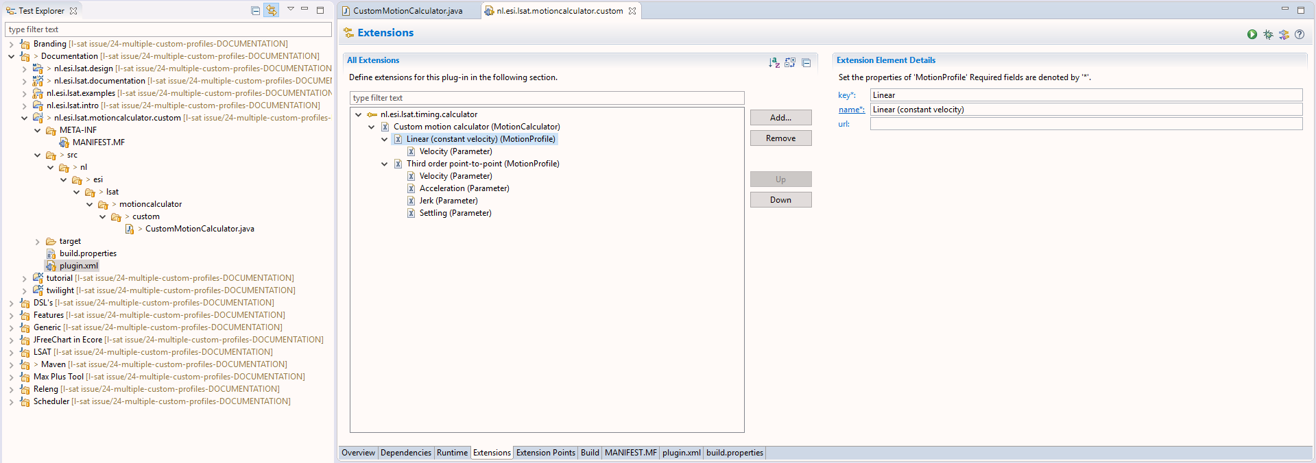 Figure 22. Example with a custom (Linear) motion profile and the default (Third order point-to-point) motion profile.
You can also modify the plugin.xml file of your motion calculator plugin to define motion profiles and parameters. Listing 1. plugin.xml showing the motion profile and parameter specifications<MotionProfile key="Linear" name="Linear (constant velocity)"> <Parameter key="V" name="Velocity" required="true"> </Parameter> </MotionProfile> <MotionProfile key="ThirdOrderP2P" defaultProfile="true" name="Third order point-to-point"> <Parameter key="V" name="Velocity" required="true"> </Parameter> <Parameter key="A" name="Acceleration" required="true"> </Parameter> <Parameter key="J" name="Jerk" required="true"> </Parameter> <Parameter key="S" name="Settling" required="false"> (1) </Parameter> </MotionProfile>1 Parameters can specified to be optional, but default values cannot be specified for these parameters. The defaults must be part of the implementation -
Select the extension point and create a motion calculator class by clicking the class:* hyperlink.
Below you can see an example of our CustomMotionCalculator class.Do not name your class MotionCalculator as it can lead to name clashes. Use a name like e.g CustomMotionCalculator. Make sure to implement the org.eclipse.lsat.timing.calculator.MotionCalculator interface and optionally extend the org.eclipse.lsat.timing.calculator.PointToPointMotionCalculator if you want your motion calculator to support the default third order point-to-point motion profile, like our CustomMotionCalculator. Listing 2. CustomMotionCalculator.java as an example of the motion calculator implementations.public class CustomMotionCalculator extends PointToPointMotionCalculator implements MotionCalculator { (1) protected static final String LINEAR_MOTION_PROFILE_KEY = "Linear"; @Override public void validate(List<MotionSegment> segments) throws MotionValidationException { (2) if (MotionSegmentUtilities.isMotionProfile(segments, THIRD_ORDER_POINT_TO_POINT_MOTION_PROFILE_KEY)) { super.validate(segments); (3) } else if (MotionSegmentUtilities.isMotionProfile(segments, LINEAR_MOTION_PROFILE_KEY)) { // Add your custom motion validations here if (segments.size() > 1) { throw new MotionValidationException( "Event-on-the-fly (move passing) is not supported by CustomMotionCalculator", segments); } if (MotionSegmentUtilities.getSettledSetPointIds(segments).size() > 0) { throw new MotionValidationException("Settling is not supported by CustomMotionCalculator", segments); } } else { throw new MotionValidationException( "Mixing motion profiles in one move is not supported by CustomMotionCalculator", segments); } } @Override public List<Double> calculateTimes(List<MotionSegment> segments) throws MotionException { (4) if (MotionSegmentUtilities.isMotionProfile(segments, THIRD_ORDER_POINT_TO_POINT_MOTION_PROFILE_KEY)) { return super.calculateTimes(segments); } // Validate method already validated that motion profile equals LINEAR_MOTION_PROFILE_KEY in this case // Validate method already validated that the segments array contains exactly 1 element return Arrays.asList(calculateLinearTime(segments.iterator().next()).doubleValue()); } @Override public Collection<PositionInfo> getPositionInfo(List<MotionSegment> segments) throws MotionException { (5) if (MotionSegmentUtilities.isMotionProfile(segments, THIRD_ORDER_POINT_TO_POINT_MOTION_PROFILE_KEY)) { return super.getPositionInfo(segments); } // Validate method already validated that motion profile equals LINEAR_MOTION_PROFILE_KEY in this case // Validate method already validated that the segments array contains exactly 1 element MotionSegment segment = segments.iterator().next(); BigDecimal segmentTime = calculateLinearTime(segment); List<PositionInfo> result = new ArrayList<>(); BigDecimal position = BigDecimal.valueOf(0); for (MotionSetPoint motionSetPoint: segment.getMotionSetpoints()) { BigDecimal setPointTime = calculateLinearTime(motionSetPoint); PositionInfo positionInfo = new PositionInfo(motionSetPoint.getId()); position = MotionSetPointUtilities.getFrom(motionSetPoint, position); positionInfo.addTimePosition(0d, position.doubleValue()); position = MotionSetPointUtilities.getFrom(motionSetPoint, position.add(motionSetPoint.getDistance())); positionInfo.addTimePosition(setPointTime.doubleValue(), position.doubleValue()); // If setPoint arrives early at To, add a third sample if (setPointTime.compareTo(segmentTime) < 0) { positionInfo.addTimePosition(segmentTime.doubleValue(), position.doubleValue()); } result.add(positionInfo); } return Collections.unmodifiableCollection(result); } private BigDecimal calculateLinearTime(MotionSegment segment) { BigDecimal maxTime = BigDecimal.ZERO; for (MotionSetPoint motionSetPoint: segment.getMotionSetpoints()) { maxTime = maxTime.max(calculateLinearTime(motionSetPoint)); } return maxTime; } private BigDecimal calculateLinearTime(MotionSetPoint motionSetPoint) { if (!motionSetPoint.doesMove()) { return BigDecimal.ZERO; } BigDecimal velocity = motionSetPoint.getMotionProfileArgument(VELOCITY_PARAMETER_KEY); return motionSetPoint.getDistance().abs().divide(velocity, 6, RoundingMode.HALF_UP); } }1 To reuse the built in default motion calculator of Eclipse LSAT™ extend your newly created class with PointToPointMotionCalculator. 2 Start with the implementation of the validate method. The constraints can be on an individual level or combined. 3 If you are reusing the PointToPointMotionCalculator, you can reuse the validate from the super class. 4 Continue with the implementation of calculateTimes. This method is called after validation. It is mandatory and its purpose is to determine the duration of the move. 5 Finally implement the getPositionInfo. This method is called after validation when a motion plot is created and calculates for each setpoint its position over time. For incremental development this function could first be left empty, till the calculator works. Additionally, getPositionInfo is used to visualizes the profile. For more info, check out Plotting a move in Chapter 3 from the user guide.
-
The motion calculator always calculates a move for a single peripheral from standstill to standstill.
-
A move consists of one or more (in case of a passing move) MotionSegments.
-
The default PointToPointMotionCalculator only supports a passing move, when for all MotionSegments the motion profile is the same and its parameter values are the same.
-
Each MotionSegment contains a MotionSetPoint for every setpoint of the peripheral.
-
A MotionSetPoint indicates where the movement comes from and where it needs to go.
Test your new motion calculator
-
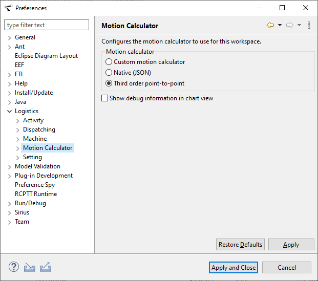
Start the Eclipse LSAT™ runtime environment from within the development environment by means of the predefined Eclipse LSAT™ launch target.
-
Select your custom motion calculator via the menu.
-
Open the .settings file of an Eclipse LSAT™ specification.
-
Go to the Axis and then Profiles section.
-
Put your mouse cursor the existing profile e.g normal.
-
Press Ctrl + Space. Select the previously defined motion profile, Linear in our code example.

-
Finish by defining the values for the parameters that the custom motion profile requires.

-
Appendix B: How to implement a custom motion calculator with Json
Eclipse LSAT™ provides a customisable API to translate specified motion profiles into duration times or time/position info.
The API is used to analyse throughput in timing analysis and to plot moves in an activity diagram.
Third parties have the possibility to implement their own Motion Calculator in their own programming language of choice using Json. This appendix describes what needs to be done for that.
Terminology
| Term | Description | Remark |
|---|---|---|
Motion profile |
A set of parameters for a motion calculator implementation to calculate times or position info. |
A motion profile can be supplied by third parties.
For example a Third order profile with parameters Velocity, Acceleration, Jerk
If more than one profile is supplied then exactly one profile must have |
Motion Segment |
Specifies a move from position A to B along one or more specified axes. Each axis movement is specified in a Motion Set Point. |
|
Motion Segment Array |
A concatenated set of moves from position to position where in between segments specify passing positions while moving. The first segment starts with velocity 0 and the last segment ends with velocity 0. This is typically called a point-to-point move. |
|
Motion Set Point |
A movement along one axis containing the from, to position or distance and the profile parameter values. |
A setpoint has an id which typically represents an axis If a motion segment contains more than one setpoint they are all moving at the same moment in time. |
Supported Profiles |
The list of one or more profiles supported by a Motion Calculator. |
|
Validate |
Validates if the given data can be handled without errors by a Motion Calculator. |
|
Calculate Times |
Calculate duration of a set of (concatenated) moves. An array with times in seconds for each motion segment is returned. The value is the delta time against beginning of the move. |
|
Get Position Info |
Get the position info per of a set of (concatenated) moves. An array containing (absolute) times (duration since start in seconds) and (absolute) position (in meter) per set point id is returned |
Json Interface
Json data is transported using a synchronous shared library function call.
Third parties should implement this function and offer it in a shared library.
#ifndef JSON_SERVER_H
#define JSON_SERVER_H

/*
   Interface call to a Motion Calculator Json server.
   See the LSAT design documentation for the json data to be exchanged.

   request contains the UTF-8 encoded  Json request data
   response is a buffer of size response_size that can be used to write
   the json response to. response must be UTF-8 encoded.

   the function should return 0 except when the response does not fit
   into the response buffer then it should return a non 0 value.

   errormessages not related to `buffer overflows` should be return into
   the json response.
*/
extern "C" int request(char* response, const char* request, size_t response_size);

#endif // JSON_SERVER_H
Configuring the shared library
The shared library can be configured in Eclipse LSAT™ preferences. Make sure the library is visible in the execution path of Eclipse LSAT™

Json Schema for request and response
The schema can be used to validate Json and/or to bind to a specific language like c, cpp, c#, ada, etc.
{
  "$schema": "http://json-schema.org/draft-04/schema#",
  "type": "object",
  "properties": {
    "requestType": {
      "type": "string",
      "enum": ["Validate", "CalculateTimes","PositionInfo","SupportedProfiles"]
    },
    "segments": {
      "type": "array",
      "items": [
        {
          "type": "object",
          "properties": {
            "setPoints": {
              "type": "array",
              "items": [
                {
                  "type": "object",
                  "properties": {
                    "id": {
                      "type": "string"
                    },
                    "from": {
                      "type": "number"
                    },
                    "to": {
                      "type": "number"
                    },
                    "distance": {
                      "type": "number"
                    },
                    "settling": {
                      "type": "boolean"
                    },
                    "motionProfileId": {
                      "type": "string"
                    },
                    "arguments": {}
                  },
                  "required": [
                    "id",
                    "distance",
                    "motionProfile"
                  ]
                }
              ]
            },
            "id": {
              "type": "string"
            }
          },
          "required": [
            "setPoints",
            "id"
          ]
        }
      ]
    }
  },
  "required": [
    "requestType"
  ]
}{
"$schema": "http://json-schema.org/draft-04/schema#",
"type": "object",
"properties": {
"requestType": {
"type": "string",
"enum": ["Validate", "CalculateTimes","PositionInfo","SupportedProfiles"]
},
"times": {
"type": "array",
"items": [
{
"type": "number"
}
]
},
"positionInfo": {
"type": "array",
"items": [
{
"type": "object",
"properties": {
"setPointId": {
"type": "string"
},
"timePositions": {
"type": "array",
"items": [
{
"type": "array",
"items": [
{
"type": "number"
},
{
"type": "number"
}
]
},
{
"type": "array",
"items": [
{
"type": "number"
},
{
"type": "number"
}
]
}
]
}
},
"required": [
"id",
"positions"
]
}
]
}
},
"motionProfiles": {
"type": "array",
"items": [
{
"type": "object",
"properties": {
"key": {
"type": "string"
},
"name": {
"type": "string"
},
"defaultProfile": {
"type": "boolean"
},
"url": {
"type": "string"
},
"parameters": {
"type": "array",
"items": [
{
"type": "object",
"properties": {
"key": {
"type": "string"
},
"name": {
"type": "string"
},
"required": {
"type": "boolean"
}
},
"required": [
"key",
"name",
"required"
]
}
]
}
},
"required": [
"key",
"name",
"parameters"
]
}
]
},
"required": [
"requestType"
]
}Examples of Json messages
Supported Profiles
{
    "requestType": "SupportedProfiles"
}
{
"requestType": "SupportedProfiles",
"motionProfiles": [
{
"key": "test",
"name": "test",
"defaultProfile": true,
"parameters": [
{
"key": "V",
"name": "V",
"required": true
},
{
"key": "A",
"name": "A",
"required": true
},
{
"key": "J",
"name": "J",
"required": true
}
]
}
]
}Validate
{
    "requestType": "Validate",
    "segments": [
        {
            "setPoints": [
                {
                    "id": "X",
                    "from": 0.3,
                    "distance": 0,
                    "settling": false,
                    "motionProfileId": "ThirdOrderP2P",
                    "arguments": {
                        "A": 0.5,
                        "S": 0.1,
                        "V": 0.5,
                        "J": 0.5
                    }
                },
                {
                    "id": "Y",
                    "from": 0.15,
                    "distance": -0.3,
                    "settling": true,
                    "motionProfileId": "ThirdOrderP2P",
                    "arguments": {
                        "A": 0.5,
                        "S": 0.1,
                        "V": 0.5,
                        "J": 0.5
                    }
                }
            ],
            "id": "nodeto A1"
        }
    ]
}
{
"requestType": "Validate"
}Calculate Times
{
    "requestType": "CalculateTimes",
    "segments": [
        {
            "setPoints": [
                {
                    "id": "X",
                    "from": 0.3,
                    "distance": 0,
                    "settling": false,
                    "motionProfileId": "ThirdOrderP2P",
                    "arguments": {
                        "A": 0.5,
                        "S": 0.1,
                        "V": 0.5,
                        "J": 0.5
                    }
                },
                {
                    "id": "Y",
                    "from": 0.15,
                    "distance": -0.3,
                    "settling": true,
                    "motionProfileId": "ThirdOrderP2P",
                    "arguments": {
                        "A": 0.5,
                        "S": 0.1,
                        "V": 0.5,
                        "J": 0.5
                    }
                }
            ],
            "id": "nodeto A1"
        }
    ]
}
{
"requestType": "CalculateTimes",
"times": [
2.777731800328678
]
}Position Info
{
    "requestType": "PositionInfo",
    "segments": [
        {
            "setPoints": [
                {
                    "id": "X",
                    "from": 0.3,
                    "distance": 0,
                    "settling": false,
                    "motionProfileId": "ThirdOrderP2P",
                    "arguments": {
                        "A": 0.5,
                        "S": 0.1,
                        "V": 0.5,
                        "J": 0.5
                    }
                },
                {
                    "id": "Y",
                    "from": 0.15,
                    "distance": -0.3,
                    "settling": true,
                    "motionProfileId": "ThirdOrderP2P",
                    "arguments": {
                        "A": 0.5,
                        "S": 0.1,
                        "V": 0.5,
                        "J": 0.5
                    }
                }
            ],
            "id": "nodeto A1"
        }
    ]
}
{
"requestType": "PositionInfo",
"positionInfo": [
{
"setPointId": "X",
"timePositions": [
[
0.0,
0.3
],
[
2.777731800328678,
0.3
]
]
},
{
"setPointId": "Y",
"timePositions": [
[
0.0,
0.15
],
[
0.4244,
0.14362992010133332
]
]
}
]
}Background Eclipse LSAT™ Internal motion calculator API
| This background is only for informational purposes. |
Internally the motion calculator API in Eclipse LSAT™ consists of 2 interfaces:
    /**
     * Validates if this {@link MotionCalculator} is able to calculate the motion as specified by <tt>segments</tt>.
     *
     * @param segments the specified motion.
     * @throws MotionException If this motion calculator is not able to calculate this motion
     */
    void validate(List<MotionSegment> segments) throws MotionValidationException;

    /**
     * Calculate the motion times for the an array of concatenated segments.<br>
     * <b>IMPORTANT:</b> The time in the array is the end-time of the motion segment measured from the start of the
     * concatenated move.
     *
     * @param segments
     * @return A list of {@link Double}s representing time in seconds where the index of the array corresponds with the
     *     index of the motion segment in the provided segment list.
     * @throws MotionException
     */
    List<Double> calculateTimes(List<MotionSegment> segments) throws MotionException;

    /**
     * Calculates the position information for all set-points in an array of concatenated segments.
     *
     * @param segments
     * @return The PositionInfo per set point.
     * @throws MotionException
     */
    Collection<PositionInfo> getPositionInfo(List<MotionSegment> segments) throws MotionException;
} /**
* Provides the supported profiles and its parameters.
*
* <p>
* MotionCalculator providers that also implement this API can expect that only supported profiles will be used
* </p>
* Example of a profile: <pre>
* {@link MotionProfile}
* key="ThirdOrderP2P"
* name="Third order point-to-point"
* url="optional url to online specification"
* {@link MotionProfileParameter} key="V" name="V" required="true"
* {@link MotionProfileParameter} key="A" name="A" required="true"
* {@link MotionProfileParameter} key="J" name="J" required="true"
* {@link MotionProfileParameter} key="S" name="S" required="false"
* </pre>
*
* @return The supported profiles for an implementation
* @throws MotionException
*/
Set<MotionProfile> getSupportedProfiles() throws MotionException;
}