TRACE Behavioral analysis
NOTE: Analysis is applied to the current filtered view
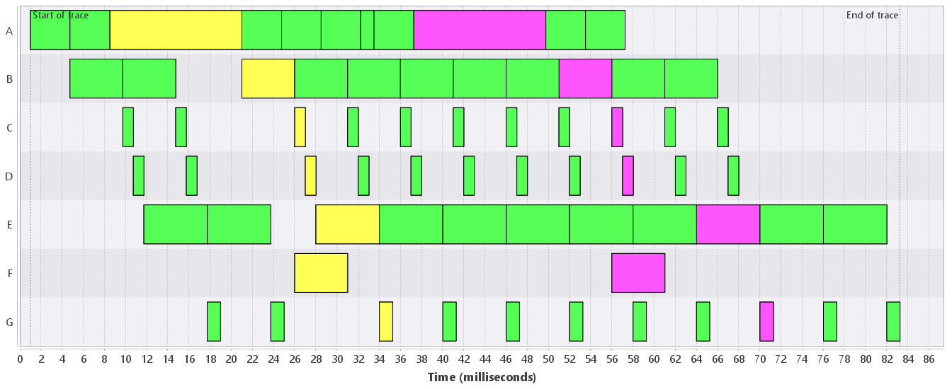
Many systems exhibit more or less repetitive behavior, e.g., video-processing pipelines and manufacturing machines such as professional printers and wafer scanners. Execution traces of such systems hence also are more or less repetitive. The running example of a video-processing system, for instance, gives highly repetitive traces, e.g., the one in Figure 1 which shows the processing of 11 frames. Disturbances in the repetitive patterns in an execution trace can hint at (performance) problems. The behavioral analysis that TRACE supports aims to find such disturbances.

The behavioral analysis works on claims. It assumed that the trace comes from a system that processes identifiable objects. The objects, for example, can be frames, sheets of paper or wafers, each with a unique identifier. The analysis thus requires that each claim has an attribute with an integer value that is the identifier of the object that is being processed. This is the object identifier attribute. In the trace of Figure 1, each claim has an attribute "id" with an integer value. The coloring is according to this "id" attribute, and "id" serves as the object identifier attribute.
The analysis first creates a partition of the claims according to the object identifier attribute: claims with the same value for the object identifier attribute are placed in the same cell of the partition. Such a cell is called a behavior. In Figure 1, all claims with identical color are a behavior (because the coloring is according to the object identifier attribute).
The analysis then compares the behaviors in a trace with each other. This is done with the pseudo metric (distance) explained here. To compare a behavior B1 with another behavior B2, the claims of B1 are used to create a trace T1 and the claims of B2 are used to create a trace T2, which are input to the distance computation. The distance computation uses as a basis for equality of vertices in T1 and T2 (i) a subset of the attributes (uniqueness attributes), and (ii) the resource that a claim uses. These uniqueness attributes are a second parameter of the analysis, next to the object identifier. In our running example, see Figure 1, we could use the "name" attribute as the uniqueness attribute. This, however, is not necessary as each claim in a behavior uses a unique resource.
The pseudo metric induces an equivalence relation on behaviors. Two behaviors are equivalent if and only if their distance equals 0. This informally means that the order of the processing steps that are modeled by the claims in the two behaviors are equal. This equivalence relation is used to create the behavioral partition. For instance, when we compare the first (cyan) behavior with the second (red) behavior in Figure 1, we get distance 0. These two behaviors are thus part of the same cell in the behavioral partition.
The behavioral analysis can be started with the menu (![]() )
and has three items:
)
and has three items:
- Behavioral classes : This analysis gives the behaviors in each cell of the behavioral partition a unique color. An example is shown in Figure 2. Apparently, the trace in Figure 1 containts three kinds of behaviors. Note that the difference is whether activity with name F is present or not, and if it is present, whether it overlaps with the activity with name E.
- Behavioral representatives : This analysis adds a filter to show only a single (random) behavior from each cell in the behavioral partition. Figure 3, for instance, shows three representatives of the different behaviors that occur in the trace.
- Behavioral histogram : This analysis shows a histogram of the sizes of the various cells in the behavioral partition. The histogram is opened in a separate view, see Figure 4.