Simulation of traces

> > >

The CIF simulator simulates one particular trace through the state space of the specification. To better understand what the previous sentence means, this page further explains each of those concepts.

State

Automata consist of one or more locations. However, at any time, an automaton can only be in one of its locations. This location is called the current or active location. The current location of an automaton is also called the state of the automaton.

Similar to having multiple locations in automata, variables usually have many possible values. However, similar to automata having only one current location, variables can not have two values at the same time.

The current location of each of the automata (i.e. the states of the automata), together with the current values of the variables (all discrete, input and continuous variables, including variable time), is called the state of the specification. The state of the specification (or simply 'the state'), is all the information that needs to be maintained about the history of the simulation, going forward.

For instance, consider the following specification:

automaton button:
  event pushed, released;

  location Released:
    initial;
    edge pushed goto Pushed;

  location Pushed:
    edge released goto Released;
end

automaton machine:
  event producing, produced;

  location Idle:
    initial;
    edge producing when button.Pushed goto Producing;

  location Producing:
    edge produced goto Idle;
end

We have two automata, button and machine. Pushing the button (event button.pushed) turns on the machine. Releasing the button (event button.released) turns it off. Initially, the machine is Idle. While the button is pushed (location button.Pushed is the current location of automaton button), the machine can start to create a product (event machine.producing). Once the machine has produced a product (event machine.produced), the machine becomes idle again. Note that once the machine starts producing a product, it always finishes producing it, even if it is turned off in the mean time.

The state of automaton button is either of its locations: button.Released or button.Pushed. Similarly, the state of automaton machine is machine.Idle or machine.Producing. Initially, the system is in state button: Released, machine: Idle, time: 0.0. For the remainder of variable time will omitted from the state, for brevity only. Furthermore, also for brevity only, we’ll omit the names of the automata. Therefore, the initial state is Released, Idle.

State space

The state space of a specification consists all the possible states of the specification, connected by the transitions via which they can be reached.

For the example above, the state space is (event names are abbreviated):

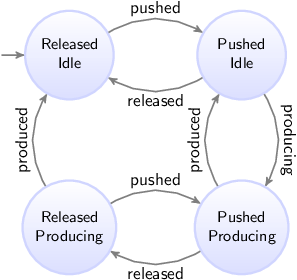
Since both automata can be in two states, the state space in this case consists of four states. From the initial state (the upper left state), the button can be pushed, leading to the upper right state, where the button is pushed, while the machine has not yet started to produce a product. The machine can then start to produce a product (going to the lower right state). If however the button is released before the machine can respond by starting to produce a product, we go back to the upper left state. When the machine finishes creation of the product, we go from the lower right state back to the upper right state. If on the other hand the button is released, while the product is still being produced, we go from the lower right state to the lower left state. If we then push the button again, we go back to the lower right state. If instead the button is not pushed, and the machine finishes producing the product, we go from the lower left state back to the upper left state.

Traces

A trace is a sequence of transitions, from the initial state, through the state space.

In state spaces, most states usually have multiple outgoing transitions. This means there is choice. That is, it is possible to choose to which next state to go. Furthermore, it is usually possible to keep taking transitions forever, which means we can have infinite traces.

For the example above, some of the possible traces are shown below. Only the first five transitions of the traces are shown. State names are abbreviated, to the first letters of the names of the locations.

RI → pushed → PI → released → RI → pushed → PI → released → RI → pushed → PI → …
RI → pushed → PI → producing → PP → produced → PI → producing → PP → produced → PI → …
RI → pushed → PI → producing → PP → released → RP → produced → RI → pushed → PI → …

In the first trace, we push the button, release it, push it again, release it, and push it again, all without ever starting to produce a product. This traces shows us what happens if the button is constantly being pushed and released, as quickly as possible, without the machine being able to respond to this, by starting to produce a product.

In the second trace, we push the button, we start to produce a product, we finish producing it, start to produce another product (the button is still pushed), finish producing the second product, and start to produce a third product. This is a trace of a typical usage scenario, where we start the machine, and the machine keeps running.

In the third trace, we push the button, start to produce a product, release the button before the product is finished, finish producing the product, and push the button again. This trace is another typical usage scenario, which also includes turning off the machine.

Simulation

As stated at the top of the page: 'The CIF simulator simulates one particular trace through the state space of the specification'. To see why this is the case, we take a look at the main simulation loop, as used by the simulator:

Calculate the initial state, and set it as the current state.
Forever, do:
- If the user-provided simulation end time is reached, stop simulation.
- Calculate the possible transitions for the current state.
- If no transitions are possible (deadlock), stop simulation.
- Choose one of the possible transitions.
- Take the chosen transition, and set its target state as the new current state.

While this main simulation loop is simplified with respect to the real implementation, it gives some insight into the inner workings of the simulator. The simulator keeps taking transitions. Once a transition is taken, the current state is updated to the target state of the transition. This means that the other possible transitions (the ones that were not chosen), are not taken. Therefore, if we want to take a different transition, we should restart simulation from the initial state, and make different choices. That is, if we want to simulate a different trace, we perform another simulation.

Validation

The simulator can be used to gain confidence in the correctness of the specification. By simulating various traces, we can observe what happens in different scenarios (use cases). Since the number of traces if often infinite, covering the entire state space, and all possible traces, is impossible. However, by wisely choosing the traces we simulate, we can cover a large part of the state space.

It should be clear by now, that simulating a single trace is almost never enough to conclude that your specification is 'correct'. Different traces lead to different behavior, and only by testing enough traces, and thus covering enough of the system’s behavior, can you conclude that your specification works as expected (for those traces).