First example
Before we go into any details about SVG visualization, let’s first look at an example. Here, we use a trivial example, which nonetheless serves several purposes:
-
It gives a quick overview of what the idea of SVG visualization is all about, and what it looks like.
-
It shows how to use SVG visualization with the CIF simulator.
-
It shows the two alternatives to simulation: via the options dialog, and by using a ToolDef script.
Note that it is not necessary to fully understand what exactly is going on, or how it works. Those details should become clear after reading the remaining pages of the documentation.
Creating the CIF model
In an Eclipse project or directory, create a new CIF file named lamp.cif:
svgfile "lamp.svg";

automaton lamp:
  cont t der 1.0;

  location Off:
    initial;
    edge when t >= 1.0 do t := 0.0 goto On;

  location On:
    edge when t >= 2.0 do t := 0.0 goto Off;

  svgout id "lamp" attr "fill" value if Off: "gray" else "yellow" end;
end
This file describes not only the behavior of the lamp using a CIF automaton, but also contains a CIF/SVG declaration, which specifies the connection between the behavioral CIF specification and the SVG image.
Creating the SVG image
Next, we’ll create an SVG image. Start Inkscape, Select , to open the Document Properties window. On the Page tab, set the Units to px, the Width to 75.00, and the Height to 100.00. It is recommended to always set the size of the image, before adding any shapes or text labels.
Next, select the circle tool, by clicking on the circle in the Toolbox on the left side of the application. Draw a circle on the canvas. It should look something like this:
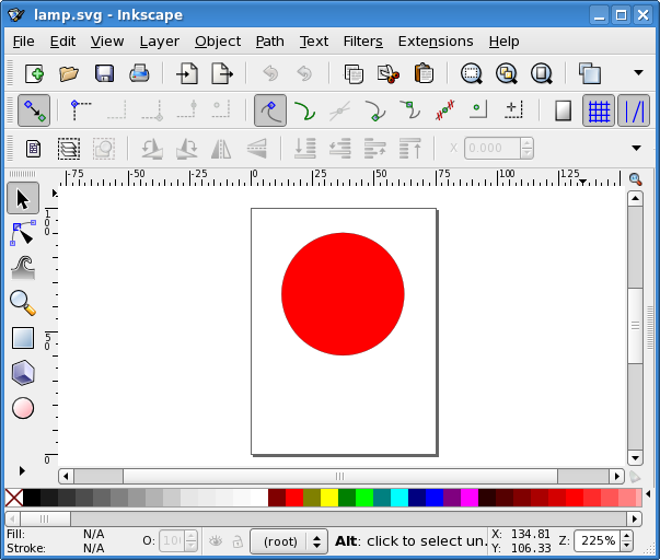
Right click the circle and choose Object Properties. The Object Properties window will appear. Change the Id of the circle to lamp and click the Set button. Save the image as lamp.svg, in the same directory as the lamp.cif file.
Simulation and the options dialog
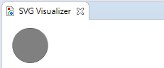
Right click the lamp.cif file and choose to start the CIF simulator. An options dialog appears. In this case the defaults suffice, so click OK to start the simulation. Initially, the visualization looks as follows:
Using the GUI input, click the button for time delay and then the button for tau. After performing these two transitions, the visualization should look as follows:
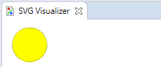
As you can see, the lamp is gray while it is off, and yellow while it is on. Close the GUI input window to terminate the simulator. You may also close the visualization window.
Now restart the simulator. In the Simulator category, set the Simulation end time option to Finite end time. You can leave the default value for End time. In the Input category, set the Input mode option to Automatic input mode. In the Output category, enable the Frame rate option and keep the default frame rate value. Click OK to start the simulation again. This time, the simulator automatically chooses transitions. Furthermore, real-time simulation is enabled, where the model time is interpreted in seconds, and the visualization is regularly updated. Using these options, SVG visualization essentially turns into an SVG movie of the simulation of a flashing lamp. Simulation will automatically stop after ten seconds, the default simulation end time. Once simulation terminates, you may close the visualization window.
Simulation using ToolDef
While the option dialog is useful for configuring simulation options, it is often easier to use a ToolDef file to script the execution of the CIF simulator. Create a new file named lamp.tooldef, in the same directory as the other files, and give it the following content:
from "lib:cif" import *;

cifsim(
    "lamp.cif",
    "-t 10",
    "-i auto",
    "--frame-rate=20",
);
Don’t forget to save the file. Right-click the lamp.tooldef file and choose Execute ToolDef to execute the ToolDef script. This script uses the exact same options as we manually configured in the option dialog, in the previous section.