Servers with time

> >

A manufacturing line contains machines and/or persons that perform a sequence of tasks, where each machine or person is responsible for a single task. The term server is used for a machine or a person that performs a task. Usually the execution of a task takes time, e.g. a drilling process, a welding process, the set-up of a machine. In this chapter we introduce the concept of time, together with the delay statement.

Note that here 'time' means the simulated time inside the model. For example, assume there are two tasks that have to be performed in sequence in the modeled system. The first task takes three hours to complete, the second task takes five hours to complete. These amounts of time are specified in the model (using the delay statement, as will be explained below). A simulation of the system should report 'It takes eight hours from start of the first task to finish of the second task'. However, it generally does not take eight hours to compute that result, a computer can calculate the answer much faster. When an engineer says ''I had to run the system for a year to reach steady-state'', he means that time inside the model has progressed a year.

The clock

The variable time denotes the current time in a model. It is a global variable, it can be used in every model and proc. The time is a variable of type real. Its initial value is 0.0. The variable is updated automatically by the model, it cannot be changed by the user. The unit of the time is however determined by the user, that is, you define how long 1 time unit of simulated time is in the model.

The value of variable time can be retrieved by reading from the time variable:

t = time

The meaning of this statement is that the current time is copied to variable t of type real.

A process delays itself to simulate the processing time of an operation with a delay statement. The process postpones or suspends its own actions until the delay ends.

For example, suppose a system has to perform three actions, each action takes 45 seconds. The unit of time in the model is one minute (that is, progress of the modeled time by one time unit means a minute of simulated time has passed). The model looks like:

proc P():
    for i in range(3):
        write("i = %d, time = %f\n", i, time);
        delay 0.75
    end
end

model M():
    run P()
end

An action takes 45 seconds, which is 0.75 time units. The delay 0.75 statement represents performing the action, the process is suspended until 0.75 units of time has passed.

The simulation reports:

i = 0, time = 0.000000
i = 1, time = 0.750000
i = 2, time = 1.500000
All processes finished at time 2.25

The three actions are done in 2.25 time units (2.25 minutes).

Adding time

Adding time to the model allows answering questions about time, often performance questions ('how many products can I make in this situation?'). Two things are needed:

Servers must model use of time to perform their task.
The model must perform measurements of how much time passes.

By extending models of the servers with time, time passes while tasks are being performed. Time measurements then give non-zero numbers (servers that can perform actions instantly result in all tasks being done in one moment of time, that is 0 time units have passed between start and finish). Careful analysis of the measurements should yields answers to questions about performance.

In this chapter, adding of passing time in a server and how to embed time measurements in the model is explained. The first case is a small production line with a deterministic server (its task takes a fixed amount of time), while the second case uses stochastic arrivals (the moment of arrival of new items varies), and a stochastic server instead (the duration of the task varies each time). In both cases, the question is what the flow time of an item is (the amount of time that a single item is in the system), and what the throughput of the entire system is (the number of items the production line can manufacture per time unit).

A deterministic system

The model of a deterministic system consists of a deterministic generator, a deterministic server, and an exit process. The line is depicted in the following figure:

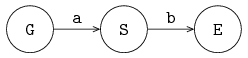
Generator process G sends items, with constant inter-arrival time ta, via channel a, to server process S. The server processes items with constant processing time ts, and sends items, via channel b, to exit process E.

An item contains a real value, denoting the creation time of the item, for calculating the throughput of the system and flow time (or sojourn time) of an item in the system. The generator process creates an item (and sets its creation time), the exit process E writes the measurements (the moment in time when the item arrives in the exit process, and its creation time) to the output. From these measurements, throughput and flow time can be calculated.

Model M describes the system:

type item = real;

model M(real ta, ts; int N):
    chan item a, b;

    run G(a, ta),
        S(a, b, ts),
        E(b, N)
end

The item is a real number for storing the creation time. Parameter ta denotes the inter-arrival time, and is used in generator G. Parameter ts denotes the server processing time, and is used in server S. Parameter N denotes the number of items that must flow through the system to get a good measurement.

Generator G has two parameters, channel a, and inter-arrival time ta. The description of process G is given by:

proc G(chan! item a; real ta):
    while true:
        a!time; delay ta
    end
end

Process G sends an item, with the current time, and delays for ta, before sending the next item to server process S.

Server S has three parameters, receiving channel a, sending channel b, and server processing time ts:

proc S(chan? item a; chan! item b; real ts):
    item x;

    while true:
        a?x; delay ts; b!x
    end
end

The process receives an item from process G, processes the item during ts time units, and sends the item to exit process E.

Exit E has two parameters, receiving channel a and the length of the experiment N:

proc E(chan item a; int N):
    item x;

    for i in range(N):
        a?x; write("%f, %f\n", time, time - x)
    end
end

The process writes current time time and item flow time time - x to the screen for each received item. Analysis of the measurements will show that the system throughput equals 1 / ta, and that the item flow time equals ts (if ta >= ts).

A stochastic system

In the next model, the generator produces items with an exponential inter-arrival time, and the server processes items with an exponential server processing time. To compensate for the variations in time of the generator and the server, a buffer process has been added. The model is depicted below:

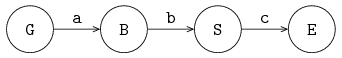
Type item is the same as in the previous situation. The model runs the additional buffer process:

model M(real ta, ts; int N):
    chan item a, b, c;

    run G(a, ta),
        B(a, b),
        S(b, c, ts),
        E(c, N)
end

Generator G has two parameters, channel variable a, and variable ta, denoting the mean inter-arrival time. An exponential distribution is used for deciding the inter-arrival time of new items:

proc G(chan item a; real ta):
    dist real u = exponential(ta);

    while true:
        a!time; delay sample u
    end
end

The process sends a new item to the buffer, and delays sample u time units. Buffer process B is a fifo buffer with infinite capacity, as described at An infinite buffer. Server S has three parameters, channel variables a and b, for receiving and sending items, and a variable for the average processing time ts:

proc S(chan item a, b; real ts):
    dist real u = exponential(ts);
    item x;

    while true:
        a?x; delay sample u; b!x
    end
end

An exponential distribution is used for deciding the processing time. The process receives an item from process G, processes the item during sample u time units, and sends the item to exit process E.

Exit process E is the same as previously, see A deterministic system. In this case the throughput of the system also equals 1 / ta, and the mean flow can be obtained by doing an experiment and analysis of the resulting measurements (for ta > ts).

Two servers

In this section two different types of systems are shown: a serial and a parallel system. In a serial system the servers are positioned after each other, in a parallel system the servers are operating in parallel. Both systems use a stochastic generator, and stochastic servers.

Serial system

The next model describes a serial system, where an item is processed by one server, followed by another server. The generator and the servers are decoupled by buffers. The model is depicted below:

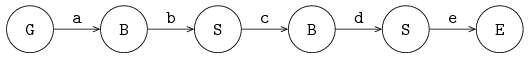
The model can be described by:

model M(real ta, ts; int N):
    chan item a, b, c, d, e;

    run G(a, ta),
        B(a, b), S(b, c, ts),
        B(c, d), S(d, e, ts),
        E(e, N)
end

The various processes are equal to those described previously in A stochastic system.

Parallel systems

In a parallel system the servers are operating in parallel. Having several servers in parallel is useful for enlarging the processing capacity of the task being done, or for reducing the effect of break downs of servers (when a server breaks down, the other server continues with the task for other items). The system is depicted below:

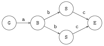
Generator process G sends items via a to buffer process B, and process B sends the items in a first-in first-out manner to the servers S. Both servers send the processed items to the exit process E via channel c. The inter-arrival time and the two process times are assumed to be stochastic, and exponentially distributed. Items can pass each other, due to differences in processing time between the two servers.

If a server is free, and the buffer is not empty, an item is sent to a server. If both servers are free, one server will get the item, but which one cannot be determined beforehand. (How long a server has been idle is not taken into account.) The model is described by:

model M(real ta, ts; int N):
    chan item a, b, c;

    run G(a, ta),
        B(a, b),
        S(b, c, ts), S(b, c, ts),
        E(c, N)
end

To control which server gets the next item, each server must have its own channel from the buffer. In addition, the buffer has to know when the server can receive a new item. The latter is done with a 'request' channel, denoting that a server is free and needs a new item. The server sends its own identity as request, the requests are administrated in the buffer. The model is depicted below:

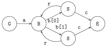
In this model, the servers 'pull' an item through the line. The model is:

model M(real ta, ts; int N):
    chan item a; list(2) chan item b; chan item c;
    chan int r;

    run G(a, ta),
        B(a, b, r),
        unwind j in range(2):
            S(b[j], c, r, ts, j)
        end,
        E(c, N)
end

In this model, an unwind statement is used for the initialization and running of the two servers. Via channel r an integer value, 0 or 1, is sent to the buffer.

The items received from generator G are stored in list xs, the requests received from the servers are stored in list ys. The items and requests are removed form their respective lists in a first-in first-out manner. Process B is defined by:

proc B(chan? item a; list chan! item b; chan? int r):
    list item xs; item x;
    list int ys; int y;

    while true:
        select
            a?x:
                xs = xs + [x]
        alt
            r?y:
                ys = ys + [y]
        alt
            not empty(xs) and not empty(ys), b[ys[0]]!xs[0]:
                xs = xs[1:]; ys = ys[1:]
        end
    end
end

If, there is an item present, and there is a server demanding for an item, the process sends the first item to the longest waiting server. The longest waiting server is denoted by variable ys[0]. The head of the item list is denoted by xs[0]. Assume the value of ys[0] equals 1, then the expression b[ys[0]]!xs[0], equals b[1]!xs[0], indicates that the first item of list xs, equals xs[0], is sent to server 1.

The server first sends a request via channel r to the buffer, and waits for an item. The item is processed, and sent to exit process E:

proc S(chan? item b; chan! item c; chan! int r; real ts; int k):
    dist real u = exponential(ts);
    item x;

    while true:
        r!k;
        b?x;
        delay sample u;
        c!x
    end
end

Assembly

In assembly systems, components are assembled into bigger components. These bigger components are assembled into even bigger components. In this way, products are built, e.g. tables, chairs, computers, or cars. In this section some simple assembly processes are described. These systems illustrate how assembling can be performed: in industry these assembly processes are often more complicated.

An assembly work station for two components is shown below:

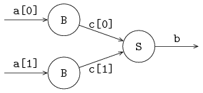
The assembly process server S is preceded by buffers. The server receives an item from each buffer B, before starting assembly. The received items are assembled into one new item, a list of its (sub-)items. The description of the assembly server is:

proc S(list chan? item c, chan! list item b):
    list(2) item v;

    while true:
        select
            c[0]?v[0]: c[1]?v[1]
        alt
            c[1]?v[1]: c[0]?v[0]
        end
        b!v
    end
end

The process takes a list of channels c to receive items from the preceding buffers. The output channel b is used to send the assembled component away to the next process.

First, the assembly process receives an item from both buffers. All buffers are queried at the same time, since it is unknown which buffer has components available. If the first buffer reacts first, and sends an item, it is received with channel c[0] and stored in v[0] in the first alternative. The next step is then to receive the second component from the second buffer, and store it (c[1]?v[1]). The second alternative does the same, but with the channels and stored items swapped.

When both components have been received, the assembled product is sent away.

A generalized assembly work station for n components is depicted below. In the figure, m = n - 1.

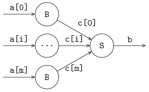
The entire work station (the combined buffer processes and the assembly server process) is described by:

proc W(list chan? item a; chan! list item b):
    list(size(a)) chan item c;

    run unwind i in range(size(a)):
            B(a[i], c[i])
        end,
        S(c,b)
end

The size of the list of channels a is determined during initialization of the workstation. This size is used for the generation of the process buffers, and the accompanying channels.

The assembly server process works in the same way as before, except for a generic n components, it is impossible to write a select statement explicitly. Instead, an unwind is used to unfold the alternatives:

proc S(list chan? item c, chan! list item b):
    list(size(c)) item v;
    list int rec;

    while true:
        rec = range(size(c));
        while not empty(rec):
            select
                unwind i in rec
                    c[i]?v[i]: rec = rec - [i]
                end
            end
        end;
        delay ...;
        b!v
    end
end

The received components are again in v. Item v[i] is received from channel c[i]. The indices of the channels that have not provided an item are in the list rec. Initially, it contains all channels 0 … size(c), that is, range(size(c)). While rec still has a channel index to monitor, the unwind i in rec unfolds all alternatives that are in the list. For example, if rec contains [0, 1, 5], the select unwind i in rec ... end is equivalent to:

select
    c[0]?v[0]: rec = rec - [0]
alt
    c[1]?v[1]: rec = rec - [1]
alt
    c[5]?v[5]: rec = rec - [5]
end

After receiving an item, the index of the channel is removed from rec to prevent receiving a second item from the same channel. When all items have been received, the assembly process starts (modeled with a delay, followed by sending the assembled component away with b!v.

In practical situations these assembly processes are performed in a more cascading manner. Two or three components are 'glued' together in one assemble process, followed in the next process by another assembly process.

Exercises

To understand how time and time units relate to each other, change the time unit of the model in The clock.
1. Change the model to using time units of one second (that is, one time unit means one second of simulated time).
2. Predict the resulting throughput and flow time for a deterministic case like in Adding time, with ta = 4 and ts = 5. Verify the prediction with an experiment, and explain the result.
Extend the model A controlled factory in Buffer exercises with a single deterministic server taking 4.0 time units to model the production capacity of the factory. Increase the number of products inserted by the generator, and measure the average flow time for
1. A FIFO buffer with control policy low = 0 and high = 1.
2. A FIFO buffer with control policy low = 1 and high = 4.
3. A LIFO buffer with control policy low = 1 and high = 4.