CIF is a declarative modeling language for the specification of discrete event, timed, and hybrid systems as a collection of synchronizing automata. The CIF tooling supports the entire development process of controllers, including among others specification, supervisory controller synthesis, simulation-based validation and visualization, verification, real-time testing, and code generation.
CIF is one of the tools of the Eclipse ESCET™ project. Visit the project website for downloads, installation instructions, source code, general tool usage information, information on how to contribute, and more.
|
The Eclipse ESCET project, including the CIF language and toolset, is currently in the Incubation Phase.
|

| You can download this manual as a PDF as well. |
The documentation consists of:
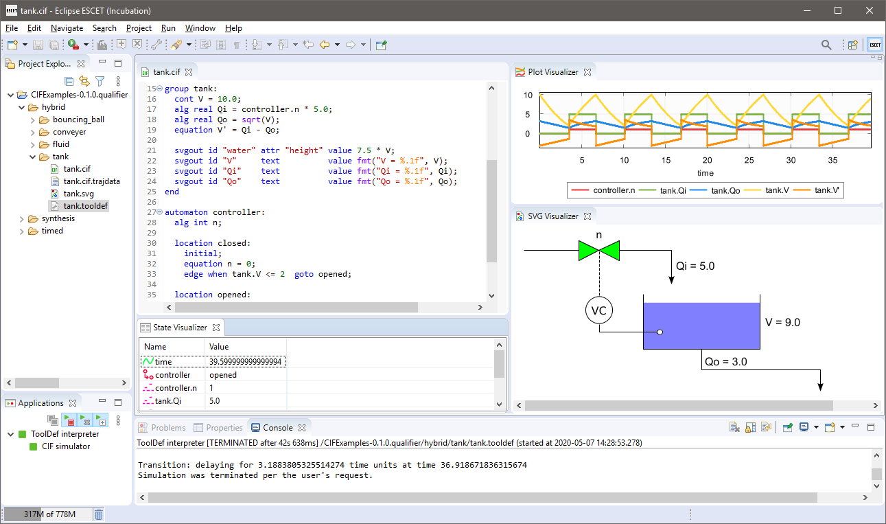
A screenshot of the CIF tooling IDE:
Introduction
The CIF language is a powerful declarative automata-based modeling language for the specification of discrete event, timed (linear dynamics), hybrid (piecewise continuous dynamics) systems. It can be seen as a rich state machine language with the following main features:
-
Modular specification with synchronized events and communication between automata.
-
Many data types are available (booleans, integers, reals, tuples, lists, arrays, sets, and dictionaries), combined with a powerful expression language for compact variables updates.
-
Text-based specification of the automata, with many features to simplify modeling large non-trivial industrial systems.
-
Primitives for supervisory controller synthesis are integrated in the language.
The CIF tooling supports the entire development process of controllers, including among others specification, supervisory controller synthesis, simulation-based validation and visualization, verification, real-time testing, and code generation. Highlights of the CIF tooling include:
-
Text-based editor that allows to easily specify and edit models.
-
Feature-rich powerful data-based synthesis tool. A transformation to the supervisory controller synthesis tool Supremica is also available.
-
A simulator that supports both interactive and automated validation of specifications. Powerful visualization features allow for interactive visualization-based validation.
-
Conversion to formal verification tools such as mCRL2 and UPPAAL.
-
Implementation language code generation (PLC languages, Java, C, and Simulink) for real-time testing and implementation of the designed controller.
Language tutorial
This tutorial introduces the CIF language. It explains the general idea behind the concepts of the language, and shows how to use them, all by means of examples. The tutorial is focused on giving a short introduction to CIF, and does not cover all details. It is recommended reading for all CIF users.
Introduction
CIF stands for Compositional Interchange Format for hybrid systems. CIF is primarily used to create models of physical systems and their controllers, describing their behavior. However, CIF is a general-purpose modeling language, and can be used to model practically anything, ranging from physical real-world systems to abstract mathematical entities.
CIF supports discrete event models, that are mostly concerned with what happens, and in which order. CIF also supports timed systems, where timing plays and explicit role, and hybrid systems, which combine the discrete events with timing. This makes CIF suitable for modeling of all kinds of systems.
The CIF tooling puts a particular focus on supporting the entire development process of controllers. However, just as the CIF language, the CIF tooling can be applied much more generally. The tooling allows among others specification, supervisory controller synthesis, simulation-based validation and visualization, verification, real-time testing, and code generation.
Lessons
Several lessons are available, grouped into the following categories:
The lessons introduce new concepts, one by one, and are meant to be read in the given order.
Basics
- Automata
-
Explains automata, locations, events, edges, transitions, and more.
- Synchronizing events
-
Explains event synchronization, enabledness, traces, and state spaces.
- Non-determinism
-
Explains multiple causes of non-determinism.
- Alphabet
-
Explains alphabets for both individual automata and entire specifications.
- Event declaration placement
-
Explains the placement of event declarations.
- Shorter notations
-
Explains several shorter notations, including self loops, declaring multiple events with a single declaration, multiple events on an edge, and nameless locations.
Data
- Discrete variables
-
Explains discrete variables, guards, and updates.
- Discrete variable value changes
-
Explains how and when discrete variables can change value.
- Location/variable duality (1/2)
-
Explains the duality between locations and variables using a model of a counter.
- Location/variable duality (2/2)
-
Explains the duality between locations and variables using a model of a lamp.
- Global read, local write
-
Explains the concepts of global read and local write.
- Monitoring
-
Explains monitoring, self loops, and monitor automata.
- Old and new values in assignments
-
Explains old and new values of variables in assignments, multiple assignments, and the order of assignments.
- The
tauevent -
Explains the
tauevent. - Initial values of discrete variables
-
Explains initialization of discrete variables, including the use of default values and multiple potential initial values.
- Initialization predicates
-
Explains initialization in general, and initialization predicates in particular.
- Using locations as variables
-
Explains the use of locations as variables.
- State (exclusion) invariants
-
Explains state (exclusion) invariants.
- State/event exclusion invariants
-
Explains state/event exclusion invariants.
Types and values
- Types, values, and expressions
-
Explains the concepts of types, values, and expressions, as an introduction for the other lessons in this category.
- Values overview
-
Provides an overview of the available values, and divides them into categories.
- Integers
-
Explains integer types, values, and commonly used expressions.
- Integer ranges
-
Explains integer ranges.
- Reals
-
Explains real types, values, and commonly used expressions.
- Booleans
-
Explains boolean types, values, and commonly used expressions.
- Strings
-
Explains string types, values, and commonly used expressions.
- Enumerations
-
Explains enumeration types, values, and commonly used expressions.
- Tuples
-
Explains tuple types, values, and commonly used expressions.
- Lists
-
Explains list types, values, and commonly used expressions.
- Bounded lists and arrays
-
Explains bounded lists, arrays, and their relations with regular lists.
- Sets
-
Explains set types, values, and commonly used expressions.
- Dictionaries
-
Explains dictionary types, values, and commonly used expressions.
- Combining values
-
Explains how to combine values of different types.
Scalable solutions and reuse (1/2)
- Constants
-
Explains the use of constants.
- Algebraic variables
-
Explains the use of algebraic variables.
- Algebraic variables and equations
-
Explains the use of equations to specify values of algebraic variables.
- Type declarations
-
Explains the use of type declarations.
Time
- Timing
-
Introduces the concept of timing.
- Continuous variables
-
Explains the use of continuous variables.
- Continuous variables and equations
-
Explains the use of equations to specify values of continuous variables.
- Equations
-
Show the use of equations for both continuous and algebraic variables, by means of an example of a non-linear system.
- Variables overview
-
Provides an overview of the different kinds of variables in CIF, and their main differences.
- Urgency
-
Explains the concept of urgency, as well as the different forms of urgency.
- Deadlock and livelock
-
Explains the concepts of deadlock and livelock.
Channel communication
- Channels
-
Explains point-to-point channels and data communication.
- Dataless channels
-
Explains
voidchannels that do not communicate any data. - Combining channel communication with event synchronization
-
Explains how channel communication can be combined with event synchronization, further restricting the communication.
Functions
- Functions
-
Introduces functions, and explains the different kind of functions.
- Internal user-defined functions
-
Explains internal user-defined functions.
- Function statements
-
Explains the different statements that can be used in internal user-defined functions.
- Functions as values
-
Explains using functions as values, allowing functions to be passed around.
Scalable solutions and reuse (2/2)
- Automaton definition/instantiation
-
Explains using automaton definition and instantiation for reuse.
- Parametrized automaton definitions
-
Explains parametrized automaton definitions.
- Automaton definition parameters
-
Explains the different kinds of parameters of automaton definitions.
- Groups
-
Explains hierarchical structuring using groups.
- Group definitions
-
Explains groups definitions and parametrized group definitions.
- Imports
-
Explains splitting CIF specifications over multiple files using imports.
- Imports and libraries
-
Explains how to create libraries that can be used by multiple CIF specifications using imports, as well as how to use imports to include CIF specifications from other directories.
- Imports and groups
-
Explains how imports and groups interact.
- Namespaces
-
Explains namespaces, and how they can be used together with imports.
- Input variables
-
Explains input variables, how they can be used for coupling with other models and systems, and their relation to imports.
Stochastics
- Stochastics
-
Introduction to stochastic distributions, which allow for sampling, making it possible to produce random values.
- Discrete, continuous, and constant distributions
-
Explains the different categories of stochastic distributions: discrete, continuous, and constant distributions.
- Pseudo-randomness
-
Explains how computers implement stochastics using pseudo-random number generators, and how this affects the use of stochastics in CIF.
Language extensions
- Supervisory controller synthesis
-
Explains how to extend a model to make it suitable for supervisory controller synthesis.
- Print output
-
Explains how to extend a model to include printing of textual output.
This documentation is currently not part of the language tutorial, but of the simulator tool documentation.
- SVG visualization
-
Explains how to extend a model to couple it to an image for visualization.
This documentation is currently not part of the language tutorial, but of the simulator tool documentation.
- SVG interaction
-
Explains how to extend a model to couple it to an image for interaction via a visualization.
This documentation is currently not part of the language tutorial, but of the simulator tool documentation.
Basics
Automata
CIF models consist of components. Each of the components represents the behavior of a part of the system. Components can be modeled as automata, which form the basis of CIF. The following CIF specification, or CIF model, shows a simple automaton:
automaton lamp:
  event turn_on, turn_off;

  location on:
    initial;
    edge turn_off goto off;

  location off:
    edge turn_on goto on;
end
The automaton is named lamp, and not surprisingly represents the (discrete)
behavior of a lamp.
Automaton lamp declares two events, named turn_on and turn_off.
Events model things that can happen in a system. They represent changes. For
instance, the turn_on event indicates that the lamp is being turned on. It
represents the change from the lamp being off to the lamp being on. The event
declaration in the lamp automaton declares two events. The event
declaration only indicates that these events exist, it does not yet indicate
when they can happen, and what the result of them happening is.
All automata have one or more locations, which represent the mutually
exclusive states of the automaton. The lamp automaton has two
locations, named on and off. Automata have an active or current
location. That is, for every automaton one of its location is the active
location, and the automaton is said to be in that location. For instance,
the lamp automaton is either in its on location, or in its off
location.
Initially, the lamp is on, as indicated by the initial keyword in the
on location. That is, the on location is the initial location of the
lamp automaton. The initial location is the active location of the
automaton, at the start of the system.
In each location, an automaton can have different behavior, specified using edges. An edge indicates how an automaton can change its state, by going from one location to another. Edges can be associated with events, that indicate what happened, and thus what caused the state change.
The lamp automaton has an edge with the turn_off event, in its on
location, going to the off location. Whenever the lamp is on, the lamp
automaton is in its on location. Whenever the lamp is turned off, the
turn_off event happens. The edge with that event indicates what the
result of that event is, for the on location. In this case the result is
that the lamp will then be off, which is why the edge goes to the off
location.
The lamp automaton can go from one location to another, as described by its
edges. This is referred to as 'performing a transition', 'taking a transition',
or 'taking an edge'. The lamp automaton can keep performing transitions.
The lamp can be turned on, off, on again, off again, etc. This can go on
forever.
Synchronizing events
The power of events is that they synchronize. To illustrate this, consider the following CIF specification:
automaton producer:
  event produce, provide;

  location producing:
    initial;
    edge produce goto idle;

  location idle:
    edge provide goto producing;
end
The automaton represents a producer that produces products, to be consumed
by a consumer. The producer automaton starts in its producing location,
in which it produces a product. Once the product has been produced, indicated
by the produce event, the automaton will be in its idle location, where
it waits until it can provide the produced product to the consumer. Once it
has provided the product to the consumer, it will once again be producing
another product. Consider also the following continuation of the above
specification:
automaton consumer:
  event consume;

  location idle:
    initial;
    edge producer.provide goto consuming;

  location consuming:
    edge consume goto idle;
end
This second automaton represents a consumer that consumes products. The
consumer is initially idle, waiting for a product from the producer.
Once the producer has provided a product, the consumer will be consuming.
Once it has consumed the product, as indicated by the occurrence of the
consume event, it will become idle again.
The specification has three events, the produce and provide events
declared in the producer automaton, and the consume event declared in
the consumer automaton. The consumer automaton, in its idle
location, has an edge that refers to the provide event declared in the
producer automaton. As such, that edge and the edge in the idle
location of the producer automaton, refer to the same event.
Synchronization
Events that are used in multiple automata, must synchronize. That is, if one of those automata performs a transition for that event, the other automata must also participate by performing a transition for that same event. If one of the automata that uses the event can not perform a transition in its current location, none of the automata can perform a transition for that event.
Now, lets take a closer look at the behavior of the producer/consumer example.
Initially, the producer automaton is in its producing location, and the
consumer automaton is in its idle location. Since the producer is
the only automaton that uses the produce event, and there is an (outgoing)
edge in its current location for that produce event, the producer can
go to its idle location by means of that event.
Both the producer and consumer use the provide event. The
producer has no edge with that event in its producing location, while
the consumer does have an edge for that event in its idle location.
Since events must synchronize, and the producer can not participate, the
event can not occur at this time. This is what we expect, as the producer
has not yet produced a product, and can thus not yet provide it to the
consumer. The consumer will have to remain idle until the producer
has produced a product and is ready to provide it to the consumer.
The producer blocks the provide event in this case, and is said to
disable the event. The event is not blocked by the consumer, and is thus
said to be enabled in the consumer automaton. In the entire
specification, the event is disabled as well, as it is disabled by at least
one of the automata of the specification, and all automata must enable the
event for it to become enabled in the specification.
The only behavior that is possible, is for the producer to produce a
product, and go to its idle location. The consumer does not participate
and remains in its idle location. Both automata are then in their idle
location, and both have an edge that enables the provide event. As such,
the provide event is enabled in the specification. As this is the only
possible behavior, a transition for the provide event is performed. This
results in the producer going back to its producing location, while at
the same time the consumer goes to its consuming location.
In its producing location, the producer can produce a product.
Furthermore, in its consuming location, the consumer can consume a
product. Two transitions are possible, and CIF does not define which one will
be performed. That is, either one can be performed. No assumptions should be
made either way. In other words, both transitions represent valid behavior, as
described by this specification. Since only one transition can be taken at a
time, there are two possibilities. Either the producer starts to
produce the product first, and the consumer starts to consume after
that, or the other way around.
Traces and state spaces
Once both transitions have been taken, we are essentially in the same situation
as we were after the producer produced a product the first time, as both
automata will be in their idle locations again. The behavior of the
specification then continues to repeat forever. However, for each repetition
different choices in the order of production and consumption can be made.
During a single execution or simulation, choices are made each time that multiple transitions are possible. The sequence of transitions that are taken is called a trace. Examples of traces for the producer/consumer example are:
-
produce→provide→produce→consume→provide→produce→consume→ … -
produce→provide→produce→consume→provide→consume→produce→ … -
produce→provide→consume→produce→provide→produce→consume→ … -
produce→provide→consume→produce→provide→consume→produce→ …
The traces end with ... to indicate that they are partial traces, that go
beyond the part of the trace that is shown. These four traces however, cover
all the possibilities for the first seven transitions.
All possible traces together form the state space, which represents all the possible behavior of a system. For the producer/consumer example, the state space is:
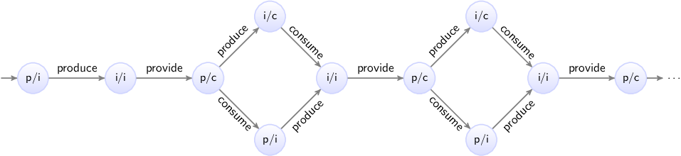
Here the circles represent the states of the specification, which are a
combination of the states of the two automata. The labels of the circles
indicate the state, as a combination of the first letters of the locations of
the automata. The initial state is labeled p/i, as initially automaton
producer is in its producing (p) location, and the consumer is in
its idle (i) location. The arrows indicate the transitions, and are labeled
with events. The state space clearly shows the choices, as multiple outgoing
arrows for a single state. It also makes it clear that as we move to the right,
and make choices, we can make different choices for different products.
Since the behavior keeps repeating itself, the state space ends with ...
to indicate that only a part of the state space is shown.
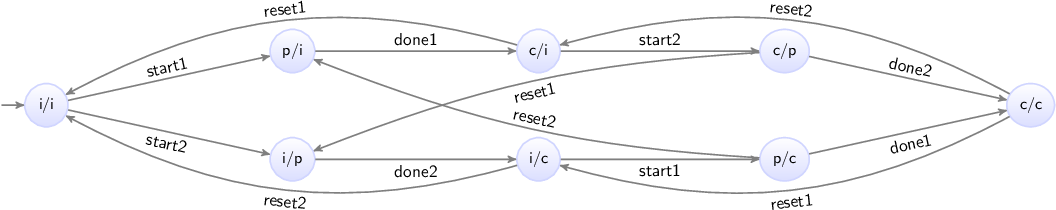
However, we can also show the entire behavior of the specification. Essential here is that the state space shown above has duplicate states. That is, several states have the same label, and allow for the same future behavior. By reusing states, a finite representation of the state space can be made, which shows the entire possible infinite behavior of the producer/consumer specification:

Concluding remarks
By using multiple automata, the producer and consumer were modeled independently, allowing for separation of concerns. This is an important concept, especially when modeling larger systems. In general, the large system is decomposed into parts, usually corresponding to physical entities. Each of the parts of the system can then be modeled in isolation, with little regard for the other parts.
By using synchronizing events, the different automata that model different parts of a system, can interact. This allows for modeling of the connection between the different parts of the system, ensuring that together they represent the behavior of the entire system.
Non-determinism
Depending on the context in which it is used, non-determinism can mean different things. One definition is having multiple possible traces through the state space of a system. Another definition is having multiple possible transitions for a certain event, for a certain state. Different communities also use different definitions, and some communities only use one of the definitions, and use a different name to refer to the other concept.
Non-determinism between events
One cause of non-determinism is that multiple events are enabled, leading to
multiple possible transitions. In other words, there are multiple possible
traces through the state space. During the lesson on
synchronizing events, we already
encountered this form of non-determinism, as transitions for the produce and
consume events could be performed in arbitrary order.
Non-determinism for single event
Another cause of non-determinism is the presence of multiple outgoing edges of a single location for the same event. This can lead to multiple possible transitions for a that event, for a single state. For instance, consider the following CIF specification:
automaton coin:
  event toss, land, pick_up;

  location hand:
    initial;
    edge toss goto air;

  location air:
    edge land goto ground;

  location ground:
    edge pick_up goto hand;
end

automaton outcome:
  location unknown:
    initial;
    edge coin.land goto heads; // First way to land.
    edge coin.land goto tails; // Second way to land.

  location heads:
    edge pick_up goto unknown;

  location tails:
    edge pick_up goto unknown;
end
The coin automaton represents a single coin. Initially, it is in the
hand of a person. That person can toss the coin up into the air,
eventually causing it to fall and land on the ground. It can be picked
up (event pick_up), causing it to once again be in the hand of a
person.
The outcome automaton registers the outcome of the
coin toss. Initially,
the outcome is unknown. Whenever the coin is tossed, it lands (event
land from automaton coin) on the ground with either the heads or
tails side up. The unknown location of the outcome automaton has
two edges for the same event. This leads to two possible transitions, one to
the heads location, and one to the tails location. This is a
non-deterministic choice, as the model does not specify which transition is
chosen, or even which choice is more likely.
In both the heads and tails locations, the coin can be picked up again,
making the outcome unknown. The coin can be tossed again and again,
repeating the behavior forever. The following figure shows the state space of
this specification:

The states are labeled with the first letters of the current locations of the two automata.
Alphabet
The lesson on synchronizing events described how events that are used in multiple automata exhibit synchronizing behavior. That is, if the event is used in multiple automata, they must all enable that event in order for a transition to be possible. If one of them can not perform the event, the event is disabled, and none of the automata can perform a transition for that event.
Whether an automaton participates in the synchronization for a certain event, is determined by its alphabet. The alphabet of an automaton is the collection of events over which it synchronizes.
Default and implicit alphabets
By default, the alphabet of an automaton implicitly contains all the events that occur on the edges of the automaton. For instance, consider the following CIF specification (the producer/consumer example from the lesson on synchronizing events):
automaton producer:
  event produce, provide;

  location producing:
    initial;
    edge produce goto idle;

  location idle:
    edge provide goto producing;
end

automaton consumer:
  event consume;

  location idle:
    initial;
    edge producer.provide goto consuming;

  location consuming:
    edge consume goto idle;
end
The alphabet of the producer automaton contains the events produce and
provide, as both occur on edges of that automaton. The alphabet of the
consumer automaton contains the events producer.produce and
consume.
Explicit alphabet
It is possible to explicitly specify the alphabet of an automaton, as follows:
event provide;

automaton producer:
  event produce;

  alphabet produce, provide; // Alphabet explicitly specified.

  location producing:
    initial;
    edge produce goto idle;

  location idle:
    edge provide goto producing;
end
The alphabet keyword is followed by the events that comprise the alphabet
of the automaton, separated by commas. In this case, the alphabet contains
the produce and provide events. Since this explicitly specified
alphabet is exactly the same as the default alphabet, it could just as easily
be omitted.
Non-default alphabet
The alphabet is allowed to be empty, which can be explicitly specified as follows:
alphabet; // Empty alphabet. Automaton doesn't synchronize over any events.However, the alphabet of an automaton must at least contain the events that occur on the edges of an automaton. That is, it must at least contain the default alphabet.
It may however also contain additional events. Since there are no edges for those additional events, the automaton can never enable those events, and thus always disables them. If a single automaton disables an event, and since it must always participate if it has that event in its alphabet, this means that the event becomes globally disabled in the entire specification. Having such additional events in the alphabet leads to a warning, to inform about the potential undesired effects of globally disabling events in this manner.
Implicit vs explicit
It should be clear that for most automata, the implicit default alphabet suffices. There are however reasons for explicitly specifying the default alphabet. For large automata, it can improve the readability, as the explicit alphabet makes it easy to determine the alphabet of the automaton, without having to look at all the edges.
The need to explicitly specifying a non-default alphabet rarely occurs. However, several tools generate CIF specifications with explicit alphabets.
Event declaration placement
Consider the following CIF specification (the producer/consumer example from the lesson on synchronizing events):
automaton producer:
  event produce, provide;

  location producing:
    initial;
    edge produce goto idle;

  location idle:
    edge provide goto producing;
end

automaton consumer:
  event consume;

  location idle:
    initial;
    edge producer.provide goto consuming;

  location consuming:
    edge consume goto idle;
end
The specification could also be specified as follows:
automaton producer:
  event produce, provide, consume; // Declaration of event 'consume' moved.

  location producing:
    initial;
    edge produce goto idle;

  location idle:
    edge provide goto producing;
end

automaton consumer:
  location idle:
    initial;
    edge producer.provide goto consuming;

  location consuming:
    edge producer.consume goto idle; // Event 'consume' from 'producer'.
end
The consume event is now declared in the producer automaton rather than
the consumer automaton, but the locations and edges have not changed. This
modified specification exhibits the same behavior as the original.
It should be clear that while events can be declared in various places, it is
best to declare them where they belong. That is, the consume event is only
used by the consumer automaton, and is thus best declared in that
automaton. Similarly, the produce event is only used by the producer
automaton.
The provide event however is used by both automata. In such cases the event
is usually declared where it is initiated. In the example above, the producer
provides the product to the consumer, and not the other way around. Therefore,
the provide event is declared in the producer automaton, rather than in
the consumer automaton.
However, the modeler is free to choose the best place to declare the event. If no choice can be made between the automata, the event can also be declared outside the automata, as follows:
event provide; // Event 'provide' now declared outside the automata.

automaton producer:
  event produce;

  location producing:
    initial;
    edge produce goto idle;

  location idle:
    edge provide goto producing;
end

automaton consumer:
  event consume;

  location idle:
    initial;
    edge provide goto consuming; // Can directly refer to 'provide' event.

  location consuming:
    edge consume goto idle;
end
This specification also has the same behavior. Only the placement of the event declarations has changed.
The place where an event is declared is of no influence to the implicit (default) alphabets of the automata. The implicit alphabet of an automaton is determined solely based on the events that occur on the edges of that automaton.
Shorter notations
This lessons explains several short notations, that can be used for easier modeling, can reduce the size of the specification, and make specifications easier to read. The following topics are discussed:
Self loop
A self loop is an edge that goes to the location from which it originated. Consider the following example:
automaton a:
  event e;

  location x:
    edge e goto x;
end
The edge in location x of automaton a goes to location x. The
effect of the e event is that automaton a remains in its x
location. A self loop can be used to allow a certain event, essentially
ignoring it for that location.
The following short notation can be used for self loops:
automaton a:
  event e;

  location x:
    edge e; // Goto omitted for self loop.
end
The goto part of the edge can be omitted for self loop. This can help make
the model easier to read, as the resulting location does not have to be checked
against the source location of the edge, to see whether they match.
Declaring multiple events with a single declaration
Several of the previous lessons already showed that multiple events can be declared using a single event declaration:
event a, b, c; // Single declaration declares multiple events.This is equivalent to using multiple event declarations that each declare a single event:
event a; // Multiple declarations each declare a single event.
event b;
event c;
Using a single declaration to declare multiple events can help reduce the length of a specification.
Multiple events on an edge
Consider the following CIF specification:
automaton a:
  event e, f;

  location loc:
    edge e goto loc; // Two edges that only differ in the event.
    edge f goto loc;
end
This can also be written more compactly, as follows:
automaton a:
  event e, f;

  location loc:
    edge e, f goto loc; // Edge with two events.
end
An edge with two or more events means exactly the same as having individual
edges for the different events. That is, a choice is made between them. It does
not specify that event f can only happen after event e has already
happened. Both automata thus have the exact same behavior.
Nameless location
Several of the examples above show automata with a single location. For such automata, the name of the location is optional:
automaton a:
  event e;

  location:
    edge e;
end
Since the location has no name, there is no way to refer to it in a goto,
and thus only self loop edges can be used. Leaving out the name prevents having
to come up with a dummy name, which can clutter the specification.
Data
Discrete variables
This lesson introduces discrete variables. Consider the following specification:
automaton counter:
  event increment, decrement;

  disc int count = 3;

  location:
    edge decrement when count > 0 do count := count - 1;
    edge increment when count < 5 do count := count + 1;
end
The counter automaton can be used to count certain things. The
increment and decrement events are used to change the count. The count
itself is stored in a variable named count. CIF has several different types
of variables. Here, we use a discrete variable, as indicated by the disc
keyword. The variable has an int data type, meaning it can have integer
numbers as its value. It is initialized to value 3.
The automaton has two edges, one for the increment event, and one for the
decrement event. The edge for the decrement event has a guard that
indicates under which circumstances the event can take place. The condition is
indicated using the when keyword. In this case, the guard ensures that the
count can only be decremented if it is currently positive. The guard of the
edge for the increment event indicates that the count can only be
incremented as long as it is less than five. In general, a guard must hold in
the source location of the edge, for the edge to be enabled, and a transition
to be possible. If the guard is not specified, it defaults to true, which
always holds and does not restrict the edge in any way.
Both edges also have updates, indicated using the do keyword. Updates can
be used to specify the effect of the transition on variables. In this case, the
updates assign a new value to the count variable that is one less or one
more than the current value. That is the value of the count variable is
decremented or incremented by one.
This specification represents a counter that can be repeatedly incremented and
decremented by one, and ensures that the value of variable count is always
at least zero and at most five.
The state space of the counter automaton is as follows:

Discrete variable value changes
Discrete variables can only change value by explicitly assigning them a new
value in the do part of an edge. If an edge does not assign a value to a
discrete variable, that variable keeps its current value. Consider the
following CIF specification:
automaton lamp:
  event turn_on, turn_off;

  disc int count = 0;

  location off:
    initial;
    edge turn_on  do count := count + 1 goto on;

  location on:
    edge turn_off                       goto off;
end
This is the same lamp automaton as used in the lesson on
automata, but with a count variable added. This
variable is used to count the number of times that the lamp has been turned on.
The edge for the turn_on event increments the value of the variable by one,
each time the lamp is turned on.
The edge for the turn_off event does not assign a value to a variable, so
variable count keeps its value when the lamp is turned off.
The state space of this specification is:

The states are labeled with the name of the current location of automaton
lamp and the current value of variable count.
Location/variable duality (1/2)
The lesson that introduces discrete variables, uses an example of a counter. The actual count was modeled using a variable:
automaton counter:
  event increment, decrement;

  disc int count = 3;

  location:
    edge decrement when count > 0 do count := count - 1;
    edge increment when count < 5 do count := count + 1;
end
It is also possible to use multiple locations instead of a variable:
automaton counter:
  event increment, decrement;

  location zero:
    edge increment goto one;

  location one:
    edge decrement goto zero;
    edge increment goto two;

  location two:
    edge decrement goto one;
    edge increment goto three;

  location three:
    initial;

    edge decrement goto two;
    edge increment goto four;

  location four:
    edge decrement goto three;
    edge increment goto five;

  location five:
    edge decrement goto four;
end
This alternate model has the same behavior, in that it models a counter that
can be incremented an decremented in steps of one, and the value is kept at
least zero, and at most five. The variant with the variable however, is shorter
and more intuitive. It is also easier to change to the count < 5 guard to
count < 100 than it is to add dozens of additional locations and edges. In
this case, using a variable is preferable to using multiple locations.
Location/variable duality (2/2)
The lesson that introduces automata, used an example of a lamp:
automaton lamp:
  event turn_on, turn_off;

  location on:
    initial;
    edge turn_off goto off;

  location off:
    edge turn_on goto on;
end
The automaton uses two locations to keep track of the current state of the lamp. Instead of two locations, it is also possible to use a variable:
automaton lamp:
  event turn_on, turn_off;

  disc bool on = true;

  location:
    initial;
    edge turn_on  when not on do on := true;
    edge turn_off when     on do on := false;
end
This alternate automaton uses a single variable named on. The
data type of the variable is
bool, which means that the variable can only have one of two possible
values: true or false. If variable on has value true, the lamp
is on, and if it has value false it is off. Initially, the lamp is on, as
the initial value of the variable is true. The automaton has only one
location, with two edges. The first edge indicates that the lamp can be turned
on (event turn_on), only when it is not currently on (guard not on),
and then afterwards is on (variable on becomes true). Similarly, the
second edge indicates that the lamp can be turned off, only when it is
currently on, and then afterwards is on.
Both models represent a lamp that is initially on, and can be turned off, on, off again, on again, etc, repeating the behavior forever. Which approach is best depends on your preference, and on the rest of the model. It is however also possible to use both locations and a variable:
automaton lamp:
  event turn_on, turn_off;

  disc bool on2 = true;

  location on:
    initial;
    edge turn_off do on2 := false goto off;

  location off:
    edge turn_on  do on2 := true  goto on;
end
This automaton has the same behavior as the previous two automata. Variable
on is renamed to on2, as a variable can not have the same name as a
location of that same automaton.
While it is possible to model a lamp like this, this automaton duplicates the information about whether the lamp is on or off. This makes the automaton larger and more complex than it needs to be. In general, it is usually better to choose either a variable, or multiple locations, to express something, and not both. In several future lessons, we’ll see that combining multiple locations with variables is useful, but not to express the same thing. Furthermore, an other future lesson explains how to use a location as a variable.
Global read, local write
Discrete variables can only be declared in automata, and may only be assigned (given a value, written) by that automaton. They may however be read globally. Consider the following CIF specification:
automaton customer:
  location:
    initial;
    edge queue1.enter when queue1.count <= queue2.count;
    edge queue2.enter when queue2.count <= queue1.count;
end

automaton queue1:
  event enter, leave;

  disc int count = 0;

  location:
    initial;
    edge enter when count < 2 do count := count + 1;
    edge leave when count > 0 do count := count - 1;
end

automaton queue2:
  event enter, leave;

  disc int count = 0;

  location:
    initial;
    edge enter when count < 2 do count := count + 1;
    edge leave when count > 0 do count := count - 1;
end
This specification models a supermarket, and features a customer and two queues. Customers arrive and enter either of the queues. Eventually customers leave the queue.
Both queues (automata queue1 and queue2) are identical, except for
their names. They maintain the count, which represents the number of
customers in the queue. A queues is full if it contains two customers.
Customers can thus only enter a queue if less than two customers are
present. Similarly, it is only possible for a customer to leave a queue if
there is a customer in the queue.
Customers decide to which queue they go, based on the number of customers already present in those queues. A customer only enters the first queue if that queue has less than or the same number of customers as the second queue. Similarly, a customer only enters the second queue if that queue has less than or the same number of customers as the first queue. If the queues have the same number of customers, the customer can choose either queue.
The enter event declared in the first queue (queue1) is used by both
the customer automaton and the queue1 automaton. The event is thus only
possible (enabled) if both automata can participate. Both automata restrict the
occurrence of the event using a guard. The event is thus only possible if both
guards hold. That is, a custom never enters the first queue if it is full, but
it also never enters that queue if it has more customers than the second queue.
The state space of this specification is as follows:
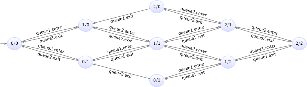
The states are labeled with the counts of the first and second queues.
The customer automaton uses the values of the variables of the queue
automata, and thus reads variables of other automata. This is allowed, due to
the global read concept of CIF. This concept allows for short guards, that
directly and intuitively represent the condition under which an event may take
place.
The global read concept should only be used when it is intuitive. In the
supermarket example, the customer can physically see how many customers are
in the queues. It is therefore intuitive to directly refer to the count
variables of the queue automata. If however the customer would not be able to
physically observer the queues, then the customer would not be able to directly
base its decision of which queue to join, on that information. In that latter
case, it may not be a good idea to model the guard in such way.
The local write concept means that discrete variables can only be written by
the automata in which they are declared. It is not allowed for the customer
and queue2 automata to write (change the value of) the count variable
of the queue1 automaton. Only the queue1 automaton may write that
variable. The local write concept prevents that multiple automata write to the
same variable, as part of a synchronizing event, potentially causing
conflicting values to be assigned to that variable. This leads to several
benefits, most notably simpler semantics.
Monitoring
This lesson explains the concept of monitoring. It is explained using the following CIF specification:
automaton producer:
  event produce, provide_a, provide_b;

  location producing:
    initial;
    edge produce goto idle;

  location idle:
    edge provide_a goto producing;
    edge provide_b goto producing;
end

automaton detect_changeover:
  disc int count = 0;

  location start:
    initial;
    edge producer.provide_a goto a;
    edge producer.provide_b goto b;

  location a:
    edge producer.provide_b do count := count + 1 goto b;

  location b:
    edge producer.provide_a do count := count + 1 goto a;
end
The producer automaton represents a producer that can repeatedly
produce a product, and provide it to either consumer 'a' (event
provide_a) or consumer 'b' (event provide_b). The consumers are not
modeled.
The detect_changeover automaton detects consumer changes. That is, it
detects and counts how often the producer switching from providing consumer 'a'
with products to providing consumer 'b' with products, and vice versa.
Initially, the automaton waits for the first product to be provided. It goes
to either location a or location b, depending on which consumer is
provided that first product. Whenever a product is then provided to the other
consumer, the count is incremented by one to account for the changeover
taking place. This also switches the location to the location for the other
consumer, where once again the automaton waits for a changeover.
The monitoring problem
There is a problem with the detect_changeover automaton. In its a
location, it disables the provide_a event, as there is no edge for that
event, and the automaton has that event in its (implicit)
alphabet. This means that after a product is
provided to consumer 'a', no more products can be provided to that same
consumer, until the producer provides a product to the consumer 'b', and the
automaton switches to the corresponding b location. However, the idea is
that the producer can provide products to either consumer, at all times, as
that is the way it is intended. The detect_changeover automaton currently
prevents behavior that is present in the producer, while it is only meant
to observe or monitor products being provided. The state space of the
specification is:

The states are labeled with the first letters of the names of the current
locations of the automata. Note how the i/a and i/b locations only have
outgoing transitions for either the provide_a transition or the
provide_b transition.
Monitoring with self loops
A simple solution is to allow the disabled events:
automaton detect_changeover:
  disc int count = 0;

  location start:
    initial;
    edge producer.provide_a goto a;
    edge producer.provide_b goto b;

  location a:
    edge producer.provide_a; // Added self loop.
    edge producer.provide_b do count := count + 1 goto b;

  location b:
    edge producer.provide_a do count := count + 1 goto a;
    edge producer.provide_b; // Added self loop.
end
The provide_a event has been added to an edge in the a location. The
edge is a self loop,
meaning the current location of automaton detect_changeover does not change
as a result of taking the edge. This means that essentially the event is
ignored by the detect_changeover automaton, as the edge also has no
updates. The state space of the modified specification is:

Now, whenever the provide_a event is possible, the provide_b event is
also possible, and vice versa, just as in the producer automaton. The
detect_changeover automaton no longer restricts the occurrence of the
events; it only monitors them.
Monitoring with monitor automata
An alternative to adding self loops, is to use a monitor automaton. A monitor
automaton is an automaton that monitors or observes one or more events. The
events that it monitors, are never blocked (disabled) by that automaton. For
our producer/changeover example, we can turn the detect_changeover
automaton into a monitor automaton for the provide_a and provide_b
events:
automaton detect_changeover:
  monitor producer.provide_a, producer.provide_b; // Monitor instead of the self loops.

  disc int count = 0;

  location start:
    initial;
    edge producer.provide_a goto a;
    edge producer.provide_b goto b;

  location a:
    edge producer.provide_b do count := count + 1 goto b;

  location b:
    edge producer.provide_a do count := count + 1 goto a;
end
By default, automata don’t monitor any events. Using a monitor declaration
with one or more events, turns the automaton into a monitor automaton for those
events. For the producer/changeover example, the behavior with the monitor
automaton is exactly identical to the behavior of the specification with the
self loops.
By omitting the events from the monitor declaration, an automaton monitors
all events of its alphabet:
monitor; // Monitor all events in the alphabet of the automaton.For the producer/changeover, which has only the provide_a and provide_b
events in its alphabet, this would result in the same behavior as for the
automaton that monitors the two events explicitly.
Using a monitor automaton instead of self loops has several advantages. A monitor declaration has to be provided only once, while self loops often have to be added to several locations. Furthermore, if the automaton is changed, it may be necessary to add or remove self loops, while the monitor declaration can most often be kept as is.
Old and new values in assignments
This lesson explains old and new values of variables in assignments, multiple assignments, and the order of assignments.
Old and new values
Consider the following CIF specification:
automaton counter:
  event increment;

  disc int count = 0;

  location:
    initial;
    edge increment do count := count + 1;
end
The counter automaton represents a counter that starts counting at zero,
and can be incremented in steps of one.
In assignments, the part to the left of the := is called the left hand
side of the assignment, or the addressable. The addressable is the variable
that is assigned, and gets the new value. In the example above, variable
count is assigned a new value.
The part to the right of the := is called the right hand side of the
assignment, or the (new) value. In the example above, the new value is
computed by taking the current or old value of variable count and
incrementing it by one.
In general, for variables used to compute the new value, always the old value of those variables are used. The new values for variables after a transition, are always computed from the old values of variables from before that transition.
Multiple assignments
It is allowed to update multiple variables on a single edge, leading to multiple variables getting a new value as part of a single transition. For instance, consider the following CIF specification:
automaton swapper:
  event swap;
  disc int x = 0, y = 0;

  location:
    initial;
    edge swap do x := y, y := x + 1;
end
The swapper automaton declares two variables, x and y. It keeps
swapping the values of both variables, each time increasing the value of y
by one.
Initially, both variables have value zero. During the first swap, variable
x gets the value of variable y. Since the old values of the variables
are used to compute the new values, variable x remains zero. Variable y
gets the old value of variable x, which is also zero, incremented by one.
The result of the first swap is that x remains zero and y becomes one.
During the second swap, x gets the value of variable y, which is then
one. Variable y gets the value of variable x, which was still zero
before the second swap, incremented by one. Both variables are thus one after
the second swap.
During the third swap, x gets the value of variable y from after the
second swap, and thus remains one. Variable y becomes two.
The state space of this somewhat artificial example is as follows:

The states are labeled with the values of variables x and y.
Assignment order
It is important to note that since the new values of the variables are computed
from the old values of the variables, assignments are completely independent of
each other. In the example above, variable x is assigned a new value in the
first assignment, and variable x is also used to compute the new value of
variable y. However, the old value of variable x is used to compute the
new value of variable y. Therefore, the assignment to x, which
indicates how x should be given a new value, has no effect on the new value
off y, as the old value of x is used for that, regardless of whether
x is assigned a new value.
Since assignments are independent of each other, the order of the assignments of the edge does not matter. Consider the following alternative edge:
edge swap do y := x + 1, x := y;The assignments to x and y have been reordered. The behavior of the
specification does not change as a result of this reordering.
Multi-assignments
CIF supports both multiple assignments as well as multi-assignments. To see the difference, consider the following examples:
edge ... do x := y, y := x + 1;     // Multiple (two) assignments.
edge ... do (x, y) := (y, x + 1);   // Single multi-assignment.
The first edge has multiple assignments, namely one assignment to variable
x and one assignment to variable y. The second edge has one assignment,
that gives new values to variables x and y. Both are identical, in that
they have the same affect: variable x is given the old value of variable
y and variable y is given the old value of variable x incremented
by one. Generally, using multiple assignments is preferred over using
multi-assignments, as the former is easier to read. However, in certain cases,
such as for tuple unpacking, only the
latter variant can be used.
Event synchronization and assignment order
Consider a system with two conveyors. Products enter on the first conveyor, and move towards the second conveyor. Once they leave the first conveyor, they move onto the second one. Once they exit from the second conveyor, they leave the system. The positions of the left sides of the boxes are in range zero to seven, as indicated in the following figure:

This system can be modeled using the following CIF specification:
event move;

automaton conveyor1:
  monitor move;
  event exit1;
  disc int pos = 0;

  location:
    initial;
    edge move  when pos < 4 do pos := pos + 1;
    edge exit1 when pos = 4 do pos := 0;
end

automaton conveyor2:
  monitor move;
  event exit2;
  disc int pos = -1;

  location:
    initial;
    edge conveyor1.exit1 when pos = -1             do pos := conveyor1.pos;
    edge move            when pos >= 0 and pos < 7 do pos := pos + 1;
    edge exit2           when pos = 7              do pos := -1;
end
Each conveyor is modeled using an automaton. Both conveyors use a pos
variable to represent the position of the left side of the box. The first
conveyor gets a new box as soon as one leaves. The second one has to wait for
a box from the first, and can thus be without a box. This is represented by
value -1 for the pos variable from automaton conveyor2. The -1
value is not a actual position, but a special value indicating that no box is
present on the conveyor.
Boxes on the first conveyor can move towards the second conveyor (event
move), until they reach position 4. They then leave the first conveyor
(event exit1), and a new box immediately enters the first conveyor
(variable pos is reset to zero).
Boxes enter the second conveyor when they leave the first conveyor (event
exit1 from conveyor1). The position of the box is then transferred from
the first conveyor to the second. The box keeps moving (event move) on
the second conveyor until it reaches position 7. At position 7 it leaves
(event exit2) the second conveyor, and the system.
Both automata synchronize over the move event, meaning that the boxes on
both conveyors move at the same time. Both automata
monitor that event to ensure it is never
blocked if only the other conveyor can actually move.
Both automata synchronize over the exit1 event. The first conveyor resets
is own position (variable pos) to zero. The second conveyor sets its own
position (variable pos) to the position of the first conveyor. Since old
values of variables are used to compute the new values, the new value of
variable pos in conveyor2 is given the old value of variable pos
from conveyor1. This is not influenced by the assignment to variable
pos of conveyor1 to zero, as assignments are independent, and the order
of assignments does not matter, just as for multiple assignments on a single
edge.
The state space of this specification is as follows:
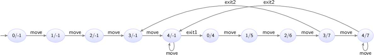
The states are labeled with the values of the pos variables of the automata
for the first and second conveyors.
The important part of the state space is the transition from state 4/-1,
where the box of the first conveyor is at the end and the second conveyor has
no box, to state 0/4, where the first conveyor has received a new box at
position zero, and the second conveyor has taken over the box (and the
administration of its position) from the first conveyor.
The tau event
Events allow for synchronization, allowing for interaction between automata based on events. If however an automaton has an edge that performs some internal processing, the event may not always be relevant. Consider for instance the following CIF specification:
automaton machine1:
  event process, provide;
  disc int id = 0;

  location processing:
    initial;
    edge process do id := id + 1 goto providing;

  location providing:
    edge provide goto processing;
end

automaton machine2:
  location:
    initial;
    edge machine1.provide;
end
The specification models two machines. Products enter the first machine,
which processes them (event process) and assigns them an id. The
machine them provides (event provide) them to the second machine. The
second machine currently just accepts the products provided by the first
machine, but would in reality likely perform its own processing as well.
The state space of the specification is as follows:

The states are labeled with the names of the current locations of automaton
machine1. Since automaton machine2 has only a single location, its
current location does not change, and it is therefore not included in the state
names.
The provide event synchronizes over both automata, while the process
event is local to the first machine. The process event is not essential,
and could be left out:
automaton machine1:
  event provide;                         // No more 'process' event.
  disc int id = 0;

  location processing:
    initial;
    edge do id := id + 1 goto providing; // No more event on the edge.

  location providing:
    edge provide goto processing;
end

automaton machine2:
  location:
    initial;
    edge machine1.provide;
end
By omitting the event from an edge, the tau is used for that edge. The
tau event is an event that is implicitly always present without declaring
it. The state space of this modified specification is:

The tau event does not synchronize. You can think of this as each automaton
having its own local tau event, and since then they are different events,
they do not synchronize. If multiple automata can perform a transition for an
edge with the tau event, this leads to potential transitions for each of
those edges. Since they are all labeled with the tau event, it is
impossible to distinguish them solely based on their label. This is a form of
non-determinism.
Using the tau events saves having to declare a local event, and also saves
having to put that event on the edge. It thus leads to smaller specifications.
However, as explained above, if tau is used on multiple edges of multiple
automata, the different tau transitions can no longer be distinguished from
each other in the state space. The use of the tau event is thus always a
trade-off.
It is also possible to explicitly use the tau event:
edge tau goto ...;The tau event can thus be used instead of 'regular' events, and may even
be combined with 'regular' events on the same edge:
edge provide, tau goto ...;
Omitting the events from an edge defaults to a single tau event, as shown
in one of the examples above.
Initial values of discrete variables
Discrete variables can be given an initial value with their declaration:
disc int x = 1;The initial value may be omitted, leading to the default value of its data type being used:
disc int x;
disc bool y;
The default value of integer typed variables
is 0. The default value of boolean typed
variables is false.
It is possible to indicate that a variable has more than one potential initial value:
disc int x in {1, 2, 4};This declares a variable x that has three potential initial values.
Variables can only have one value at a time, so an initial value has to be
chosen from the set of potential initial values.
In other words, initially the value of variable x is either 1, 2,
or 4. For information on how to store multiple values in a single variable,
see the lessons on types and values, in particular those on
tuples, lists,
and sets.
It is also possible to indicate that a variable can have any arbitrary initial value:
disc int x in any;
disc bool y in any;
Variable x can initially have any value. The only constraint is that the
initial value must be an integer value, as it must conform to the integer type
(int) of the variable. Examples of initial values include -1027,
0, 1, and 12345. Variable y can initially have any value, as
long as that value is a boolean value, due to the variable having a boolean
type (bool). There are only two boolean values, true and false.
Discrete variables with multiple potential initial values and arbitrary initial values essentially parametrize the specification. The exact initial value is to be chosen or configured later on. This allows a single specification to be used for various different combinations of initial values.
So far all examples used literal values to initialize the variables. However, it is also allowed to use expressions to compute initial values, for instance based on the initial values of other variables:
disc int x = 1;     // Initial value: 1
disc int y = x * 2; // Initial value: 2
disc int z = x + y; // Initial value: 3
Variable x is explicitly initialized with value 1. Variable y is
initialized to the initial value of x, multiplied by two. Variable z
is initialized to the sum of the initial values of x and y. Using this
kind of initialization is useful if the initial values must be kept consistent.
Changing the initial value of x automatically also changes the initial
values of y and z.
The order of the declaration of the variables does not matter. We could just as easily declare them as follows:
disc int y = x * 2; // Uses variable x, which is declared later.
disc int x = 1;
Variable y is still initialized using the initial value of variable x,
which is now declared after variable y. It is not allowed to construct
loops, where the initial values of variables depend on each other:
disc int x = y; // Invalid initial value due to cyclic dependency.
disc int y = z;
disc int z = x;
Variable x uses the value of variable y, which uses the value of
variable z, which in turn uses the value of variable x again. This is
not allowed in CIF, as it creates a cyclic dependency. However, since no
restrictions are introduced on the initial values of variables x, y,
and z, except that they must be equal to each other, we can declare them
as follows:
disc int x in any; // Explicit 'any' breaks the cyclic dependency.
disc int y = z;
disc int z = x;
Here, variable x is explicitly initialized to an arbitrary value. The other
variables are initialized to be equal to whatever arbitrary value is chosen as
initial value for variable x.
Initialization predicates
Initialization predicates can be used to specify the allowed initial locations of automata, as well as to restrict the allowed initial values of variables.
Initial locations of automata
Initialization predicates can be used to specify the allowed initial locations of automata:
automaton a:
  location loc1:
    initial;

  location loc2:
    initial true;

  location loc3;

  location loc4:
    initial false;
end
Automaton a has four locations. Location loc1 has the initial
keyword, and is thus allowed to be the initial location. Location loc2
also uses the initial keyword, but additionally specifies a predicate that
indicates under which conditions the location may be the initial location.
Since it is true, which always holds, it does not impose any additional
restrictions, and can thus always be the initial location. In fact, this is
identical to location loc1, which did not specify a predicate, in which
case it default to true as well.
Location loc3 does not specify anything about initialization, and thus
can never be the initial location. Location loc4 can only be the initial
location if false holds. Since false never holds, location loc4
can never be the initial location. In fact, this is identical to location
loc3, which did not specify any initialization at all, in which case it
default to false as well.
Locations loc1 and loc2 are the potential initial locations,
while locations loc3 and loc4 can not be chosen as initial locations of
automaton a. Since an automaton can only have one current location, an
initial location has to be chosen from the potential initial locations. In
other words, the initial location of automaton a is either location
loc1 or location loc2.
Consistency between initial locations and initial values
Consider the following CIF specification:
automaton odd_even:
  event inc, dec;
  disc int n = 5;

  location odd:
    initial;
    edge inc do n := n + 1 goto even;
    edge dec do n := n - 1 goto even;

  location even:
    edge inc do n := n + 1 goto odd;
    edge dec do n := n - 1 goto odd;
end
Automaton odd_even keeps track of a value (n) that can constantly be
incremented (event inc) and decremented (event dec) by one. It has two
locations, that keep track of the odd/even status of value n.
Currently, the initial value is 5, which is odd. Therefore, the initial
keyword is specified in the odd location. However, if we change the initial
value of variable n to 6, we have to change the initial location
as well, to ensure consistent initialization. To automatically keep the initial
location consistent with the initial value of variable n, we can change
the specification to the following:
automaton odd_even:
  event inc, dec;
  disc int n = 5;

  location odd:
    initial n mod 2 = 1; // Initial location if 'n' is odd.
    edge inc do n := n + 1 goto even;
    edge dec do n := n - 1 goto even;

  location even:
    initial n mod 2 = 0; // Initial location if 'n' is even.
    edge inc do n := n + 1 goto odd;
    edge dec do n := n - 1 goto odd;
end
In this specification, location odd can only be the initial location if
the value is odd (the value
modulo
two is congruent to
one), and location even can only be the initial location if the value is
even. Changing the initial value of variable n then also changes the
potential initial locations. Since the value is always odd or even, and can’t
be both odd and even, automaton odd_even always has exactly one potential
initial location.
Restricting initialization
Initialization predicates can also be used to restrict the initial values of variables. Consider the following CIF specification:
automaton a:
  disc int x in any;

  initial x mod 2 = 1;

  location ...
end
In this partial automaton, variable x can be initialized to any integer
value, as indicated by its int type and the any keyword. However, the
initialization predicate states that initially, the value of x module two
must be congruent to one. That is, the value of variable x must initially
be odd.
It is allowed to specify initialization predicates inside automata, but it is also allowed to place them outside of them:
automaton a:
  disc int x in any;

  location ...
end

automaton b:
  disc int x in any;

  location ...
end

initial a.x = 2 * b.x;
Here, two automata each declare a variable that can have arbitrary initial
values. The initialization predicate specifies that the initial value of
variable x from automaton b must be twice the initial value of
variable x from automaton a.
It is generally recommended to place an initialization predicate inside an automaton if the condition only applies to declarations from that automaton, and to place it outside of the automata if the condition applies to declarations of multiple automata.
Using locations as variables
Consider the following CIF specification:
automaton machine1:
  event start1, done1, reset1;
  disc bool claimed = false;

  location idle:
    initial;
    edge start1 when not machine2.claimed do claimed := true goto processing;

  location processing:
    edge done1 do claimed := false goto cool_down;

  location cool_down:
    edge reset1 goto idle;
end

automaton machine2:
  event start2, done2, reset2;
  disc bool claimed = false;

  location idle:
    initial;
    edge start1 when not machine1.claimed do claimed := true goto processing;

  location processing:
    edge done1 do claimed := false goto cool_down;

  location cool_down:
    edge reset1 goto idle;
end
This specification models two machines, which produce products. The machines
share a common resource, which may only be used by at most one of them, at any
time (see
mutual exclusion).
Initially, the machines are idle. Then, they warm themselves up. Once they
start processing, they set their boolean variable claimed to true to
indicate that they claimed the shared resource. After processing, the machines
release the resource, by setting claimed to false. They finish their
processing cycle by cooling down, before starting the cycle for the next
product. To ensure that a machine can not claim the resource if the other
machine has already claimed it, the edges going to the processing locations
have a guard that states that it is only allowed to claim the resource and
start processing, if the other machine has not already claimed the resource.
The state space of this specification is:
The states are labeled with the first letters of the names of the current locations of the automata.
The specification can alternatively be modeled as follows:
automaton machine1:
  event start1, done1, reset1;

  location idle:
    initial;
    edge start1 when not machine2.processing goto processing;

  location processing:
    edge done1 cool_down;

  location cool_down:
    edge reset1 goto idle;
end

automaton machine2:
  event start2, done2, reset2;

  location idle:
    initial;
    edge start1 when not machine1.processing goto processing;

  location processing:
    edge done1 cool_down;

  location cool_down:
    edge reset1 goto idle;
end
The claimed variables and corresponding updates have been removed, and the
guards no longer use those variables. Instead, the edge for the start1
event now refers to the processing location of automaton machine2. The
guard states that the first machine can perform the start1 event, only if
the second machine is not currently in its processing location. In other
words, the guard states that the first machine can start processing as long as
the second machine is not currently busy processing (and thus using the shared
resource).
The processing location of automaton machine2 is used as a boolean
variable. Using the location as a variable saves having to declare another
variable (claimed) that essentially holds the same information, and needs
to be explicitly updated (on two separate edges) to the correct value.
State (exclusion) invariants
The lesson on discrete variables used the following CIF specification:
automaton counter:
  event increment, decrement;

  disc int count = 3;

  location:
    initial;
    edge decrement when count > 0 do count := count - 1;
    edge increment when count < 5 do count := count + 1;
end
The counter can repeatedly be incremented and decremented by one, as long as
the count remains at least one and at most five. To keep the count in the
allowed range of values, guards were used to limit the occurrence of the
increment and decrement events.
Instead of using guards, it is also possible to use state (exclusion) invariants, also called state invariants, or just invariants:
automaton counter:
  event increment, decrement;

  disc int count = 3;

  invariant count >= 0;                   // Added invariants
  invariant count <= 5;

  location:
    initial;
    edge decrement do count := count - 1; // No more guards
    edge increment do count := count + 1;
end
The guards on the edges have been replaced by the two invariants. The first
invariant specifies that the value of variable count must always be at
least zero. The second invariant specifies that the value must also be at most
five.
Invariants specify conditions that must always hold. Invariants must hold in the initial state, and all states reached via transitions. If a transition results in a state where an invariant doesn’t hold, the transition is not allowed and can’t be taken.
For the counter example, initially the count is 3. The edge for the
increment event can be taken, leading to a state where the count is
4. Taking another transition for the increment event leads to a state
where the count is 5. If we then were to take another transition for
the increment event, the count would then become 6. However, that
violates the invariant. Therefore, in the state where the count is 5,
no transition for the increment event is possible. In other words, the
invariant disables the transition for the increment event for that state.
The two invariants can be specified in various ways:
// Multiple invariants, each with a single predicate.
invariant count >= 0;
invariant count <= 5;

// Single invariant, with multiple predicates.
invariant count >= 0, count <= 5;

// Single invariant, with single predicate.
invariant count >= 0 and count <= 5;
Each of these variants leads to the exact same behavior, and which variant to use depends mostly on the modeler’s own preference.
The benefit of guards over invariants is that they more explicitly state the condition under which an edge can lead to a transition. If a guard doesn’t hold, the edge can’t be part of a transition. It is thus immediately clear when the edge can lead to a transition. For invariants, the update has to be calculated first, after which the invariants can be evaluated for the state resulting from the transition. If one of the invariants doesn’t hold, the transition is not allowed. In the case of the invariants, it is not as immediately clear from the edge alone, when that specific edge can or can not lead to a transition.
The benefit of invariants over guards is that they apply to all edges. If several edges in an automaton have updates to the same variable, then the invariants need to be specified only once, and apply to all transitions, for all edges. Using guards, all the edges that modify the variable would need their own guards, and if the updates are different, the different edges usually require different guards. Furthermore, if new edges with updates to the same variables are added, the invariant is already present, but guards have to be added, which can easily be forgotten. In those cases, invariants can thus help keep the specification consistent.
Another benefit of invariants is that they explicitly state the conditions that must hold in relation to the variables, while guards specify the condition under which the update is allowed. Consider the following CIF specification:
// Using invariants.
automaton a:
  disc int x;

  invariant 0 <= x, x <= 100;

  location:
    initial;
    edge do x := 2 * x + 3;
end

// Using guards.
automaton a:
  disc int x;

  location:
    initial;
    edge when x <= 48 do x := 2 * x + 3;
end
The goal is to keep the value of in the range [0..100]. The invariant is simple and direct. The guard however, has to state the condition under which the update does not violate the goal. That is, the upper bound has to be decreased by three, and the result has to be divided by two, to get the highest value (48) for which the update is still within the valid range of values. That is, for value 48 the update results in value 99 (2 * 48 + 3 = 99), and for value 49 the update results in value 101 (2 * 48 + 3 = 99). The more complex the update, the harder it is to figure out the guard to use to keep satisfy the goal.
You can of course also use 2 * x + 3 <= 100 as guard, instead of
x <= 48. However, this duplicates part of the update in the guard.
So far, all invariants have been specified in automata. They may however also be specified outside of the automata, similar to initialization predicates. It is generally recommended to place an invariant inside an automaton if the condition only applies to declarations from that automaton, and to place it outside of the automata if the condition applies to declarations of multiple automata.
Furthermore, invariants can be placed in a location. Such an invariant only has to hold while the location in which it is specified is the current location of its automaton.
State/event exclusion invariants
Consider an elevator, consisting of three parts: a motor to make the elevator move up and down, a door that can be opened and closed to let passengers enter and exit, and an emergency button that can be used to stop the elevator in case of an emergency. The following CIF specification models the three parts:
automaton motor:
  event turn_on, turn_off;

  location off:
    initial;
    edge turn_on goto on;

  location on:
    edge turn_off goto off;
end

automaton door:
  event open, close;

  location closed:
    initial;
    edge open goto opened;

  location opened:
    edge close goto closed;
end

automaton emergency_button:
  event push, release;

  location released:
    initial;
    edge push goto pushed;

  location pushed:
    edge release goto released;
end
Each part is modeled by an automaton. Since the automata don’t share any events, they operate independently. What is missing, is a controller that links the different automata, and controls them in a safe manner. Such a controller restricts the behavior of the individual automata, allowing only the combined behavior that is deemed desired. There are several ways to restrict events, including introducing synchronization between the different automata, and adding guards. The downside of these approaches it that they require modification of the automata. What if we wanted to specify the controller separately from the behavior of the physical system? We could introduce an additional automaton, that synchronizes with the existing automata. For instance, we could add the following to the CIF specification:
automaton controller:
  location:
    initial;
    edge motor.turn_on when door.closed and emergency_button.released;
end
This controller introduces restrictions for the turn_on event of the
motor. In this particular case, the controller ensures that the motor may
only be turned on when both the door is closed and the emergency button is
released. By restricting the event, the controller prohibits the event from
taking place in certain states, ensuring that only the desired behavior
remains.
It is nice that we can separate the description of the physical behavior of the elevator from the controller that controls it. This separation of concerns may make it easier to reason about the behavior, it may make it easier to adapt the controller when the physical system doesn’t change, and it may make it easier to reuse the model of the physical system for other purposes.
However, modeling an automaton with a single location that must then also be
initial requires quite some syntax. State/event exclusion invariants can
serve the same purpose, but are often easier to use, shorter to write, and
more intuitive to read. Instead of the controller automaton, we can also
use the following:
invariant motor.turn_on needs door.closed and emergency_button.released;Each state/event exclusion invariant restricts an event, preventing it from
happening in certain states. That is, the event is excluded from taking place
in certain states. In this case, the turn_on event of the motor
automaton needs the door to be in its closed location and the
emergency_button to be in its released location, for the event to be
allowed/enabled. For the states in which that condition doesn’t hold, the event
is disabled.
The invariant consists of two conditions. It can also be written as two separate state/event exclusion invariants, one for each condition:
// Single state/event exclusion invariant.
invariant motor.turn_on needs door.closed and emergency_button.released;

// Multiple state/event exclusion invariants.
invariant motor.turn_on needs door.closed;
invariant motor.turn_on needs emergency_button.released;
The second and third invariants lead to the same behavior as the first combined invariant. The second invariant ensures that the event can only take place when the door is closed, while the third invariant ensures that the event can only take place when the emergency button is released. The second and third invariants each indicate a necessary condition that must hold for the event to be allowed/enabled. Together, they require that both conditions hold, for the event to be allowed/enabled. If one of the conditions doesn’t hold, the event will be disabled.
The door is either opened or closed. So far, we’ve required that
the door is closed to allow the motor to be turned on. We can also specify it
the other way around: to disallow the motor to be turned on, while the door is
opened:
// State/event exclusion invariant to specify when event is allowed/enabled.
invariant motor.turn_on needs door.closed;

// State/event exclusion invariant to specify when event is disallowed/disabled.
invariant door.opened disables motor.turn_on;
Both invariants have the exact same effect. The first invariant only allows the motor to be turned on while the door is closed, which means that it disallows the motor to be turned on in all other situations, namely when the door is opened. And that is exactly what is specified by the second invariant: when the door is opened, turning the motor on is disallowed/disabled. In general, state/event exclusion invariants can always be specified as a positive form (allowed/enabled) and a negative form (disallowed/disabled). It is up to the modeler to choose, based on considerations such as personal preference and readability. Consider the following four alternative forms:
// Single state/event exclusion invariant for enabling the event.
invariant motor.turn_on needs door.closed and emergency_button.released;
// Multiple state/event exclusion invariants for enabling the event.
invariant motor.turn_on needs door.closed;
invariant motor.turn_on needs emergency_button.released;// Single state/event exclusion invariant for disabling the event.
invariant door.opened or emergency_button.pushed disables motor.turn_on;// Multiple state/event exclusion invariants for disabling the event.
invariant door.opened disables motor.turn_on;
invariant emergency_button.pushed disables motor.turn_on;Each of the four forms has the exact same effect, but is written in a different way.
We already saw earlier that for state/event exclusion invariants that
introduce necessary conditions for an event to be enabled (the needs
variant), the conditions can be combined using an and operator to form a
combined condition, for a single invariant.
Here, we also see how in a similar way, state/event exclusion invariants that
introduce sufficient conditions for an event to be disabled (the disabled
variant) can be combined. Each of them individually has a condition, that if
satisfied disables the event, regardless of the other invariants. So, if one of
them disables the event, the event is disabled. To combine such invariants into
a single invariant, the conditions need to be combined using an or
operator, as shown above.
It may occur that multiple events need to be disabled for the same conditions. Instead of writing multiple invariants with the same conditions, one for each event, they can also be combined:
// Two separate invariants with same condition, for different events.
invariant motor.turn_on needs emergency_button.released;
invariant door.close    needs emergency_button.released;

// Combined invariant, for multiple events.
invariant {motor.turn_on, door.close} needs emergency_button.released;
The first two invariants have the same condition, but restrict different
events. The third invariant has the same condition, but restricts both events.
In general, for all state/event invariants, multiple events may be given, if
they share the same condition. The events must then be separated by spaces and
be enclosed in curly brackets ({...}).
Types and values
Types, values, and expressions
This lesson explains the difference between types, values, and expressions. These concepts have already been used in previous lessons, but this lesson names them explicitly, and also explains the relations between them. Furthermore, this lesson serves as an introduction for the coming lessons, which rely heavily on these concepts. Consider the following declarations of discrete variables:
disc int x = 1;
disc int y = 2 * x;
The first declaration declares a discrete variable named x, and the second
declaration declares a discrete variable named y. Both variables have an
int data type. A data type is usually just called a type, if there is
no confusion with other kinds of types. The type of a variable indicates the
potential or allowed values of the variable. Variable x is initialized to
value 1. Variable y is initialized to twice the value of x,
meaning it is initialized to value 2.
Both 1 and 2 * x are expressions. Expressions are combinations of
among others literal values (e.g. 1), variables (e.g. x), and
operations (e.g. *) on them. Expressions can be computed, resulting in a
value. This is called evaluation of the expression.
Expression 2 * x can be evaluated. Evaluating the expression results in
value 2 if the value of x is 1, and in value 4 if the value of
x is 2. Expressions can thus be evaluated to different values,
depending on the values of the variables that occur in them.
Expression 1 consists of only a single value, called a literal value
expression. Evaluation always results in that single value. Expression
1 + 3 evaluates to value 4. Even though it does not consist of only
just a literal, the value is the same for each evaluation. The expression
represents a constant value.
Values overview
The values of CIF (and their types) can be categorized into different categories: elementary values, container values, and miscellaneous values. Elementary values represent single values, such as a single number. Container values represent multiple values. The different container values combine or store the values in different ways. The elementary and container values are described in the remainder of this part of the tutorial. The miscellaneous values are special, and are explained later in the tutorial. The remainder of this lesson gives an overview of the values available per category, along with short descriptions of each of the different kinds of values.
Elementary values
- Booleans
-
Represents truth values of for instance guards and other conditions. The only two possible values are
trueandfalse. - Integers
-
Represent integer numbers, such as
-123and5. - Enumerations
-
Represent enumerated values, which are collections of names each representing a different value. For instance, a enumeration named
colorcould have valuesred,green, andblue. - Reals
-
Represent real numbers, such as
1.56and-2.7e6(scientific notation for 2.7 million). - Strings
-
Represent textual values, such as
"hello world"and"some text".
Container values
- Tuples
-
Tuples have two or more ordered values, each of which can have a different type. For instance:
(1, true, 5.0). - Lists
-
Lists have zero or more ordered values, each of which has the same type, and possibly with duplicates. For instance:
[1, 5, 2, 1]. - Sets
-
Sets have zero or more unordered values, each of which has the same type, and without any duplicates. For instance:
{1, 5, 2}. - Dictionaries
-
Dictionaries have keys and associated values. The keys are unique and each map to a value. For instance:
{1: true, 2: false, 3: false}.
Miscellaneous values
- Functions
-
Functions take values and use them to compute other values, possibly using complex and lengthy calculations.
- Distributions
-
Stochastic distributions allow for sampling, making it possible to produce random values.
Integers
Integers are whole numbers, numbers without a fractional part. Examples include
-123 and 5. The default value of integers (int type) is 0.
Several standard arithmetic operators and functions are available to work with
integers, including the following:
+9          // 9
--9         // 9

9 + 4       // 13
9 - 4       // 5
9 * 4       // 36
9 / 4       // 2.25 (result is a real number, not an integer number)

9 div 4     // 2    (9 / 4 = 2.25, so 4 fits at most two whole times in 9)
9 mod 4     // 1    (the remainder of 9 div 4)

pow(2, 4)   // 16   (2 to the power of 4, or 2 * 2 * 2 * 2)
abs(-9)     // 9    (absolute value)
min(9, 4)   // 4    (minimum value)
max(9, 4)   // 9    (maximum value)
Integer values can be compared to other integer values:
x < y       // less than
x <= y      // less than or equal to
x = y       // equal to
x != y      // not equal to
x >= y      // larger than or equal to
x > y       // larger than
Integer ranges
CIF can only represent integer numbers
(type int) in the range -2,147,483,648 (= -231) to
2,147,483,647 (= 231 - 1). Using values outside that range
results in the CIF model being invalid, and leads to runtime errors:
ERROR: Integer overflow: 9999999 * 9999999.It is possible in CIF to explicitly specify that only a sub range of the integer values are allowed:
disc int[3..7] x;
This variable x can only have integer values that are at least 3 and
at most 7. Assigning any other value to x is not allowed. The default
value is not 0 but 3, as that is the value closest to 0 that is in
the allowed range of values.
Reals
Reals or real numbers are numbers with a fractional part. Examples include
1.56 and -2.7e6 (scientific notation for 2.7 million). Real numbers
must either have a fraction or use the scientific notation, to distinguish them
from integer numbers. The default value of reals (real type) is 0.0.
Several standard arithmetic operators and functions are available to work with
reals, including the following:
+1.23           // 1.23
--1.2           // 1.2

1.5 + 0.5       // 2.0
1.5 - 0.5       // 1.0
1.5 * 0.5       // 0.75
1.5 / 0.5       // 3.0

pow(3.5, 2.0)   // 7.0      (3.5 to to the power of 2, or 3.5 * 3.5)
abs(-1.5)       // 1.5      (absolute value)
min(1.5, 0.5)   // 0.5      (minimum value)
max(1.5, 0.5)   // 1.5      (maximum value)

sqrt(16.0)      // 4.0      (square root)
cbrt(16.0)      // 2.0      (cube root)

sin(1.0)        // 0.841... (sine)
cos(1.0)        // 0.540... (cosine)
tan(1.0)        // 1.557... (tangent)

log(100.0)      // 2.0      (logarithm to base 10)
ln(100.0)       // 4.605... (natural logarithm)
Real values can be compared to other real values, as well as to integer values:
x < y       // less than
x <= y      // less than or equal to
x = y       // equal to
x != y      // not equal to
x >= y      // larger than or equal to
x > y       // larger than
Integer numbers can often be written where real numbers are expected. Real values and integer values can also often be combined using arithmetic operators and functions. Furthermore, it is possible to convert between them, e.g as follows:
sqrt(16)    // 4.0 (16 interpreted as 16.0)
1 + 0.5     // 1.5 (addition of an integer number and a real number)
max(0.5, 1) // 1.0 (maximum of an integer number and a real number)

<real>1     // 1.0 (cast from integer to real, explicit conversion)
round(1.6)  // 2   (round real to closest integer, half up)
ceil(0.7)   // 1   (round real up to integer)
floor(0.7)  // 0   (round real down to integer)
Booleans
Booleans represents truth values of for instance guards and other conditions
and properties. The only two possible values are true (condition or
property holds) and false (condition or property does not hold). The
default value of booleans (bool type) is false. Several standard
logical operators
are available to work with booleans, including the following:
not x       // inverse

x and y     // conjunction (both x and y must hold)
x or y      // disjunction (either x, y, or both must hold)
x => y      // implication (if x holds, y must hold)

x = y       // equal to
x != y      // not equal to
The condition x < 3 evaluates to true if x is less than 3 and
to false if x is 3 or larger than 3. The result is thus a
boolean value.
Conditions can be combined. x >= 3 and x <= 9 means that the value of x
must be both at least 3 and at most 9. x >= 3 or x <= 9 means that
the value of x must be at least 3, at most 9, or both. Since the
condition is always satisfied (it always evaluates to true), condition
true can be used instead of x >= 3 or x <= 9.
Strings
Strings represent textual values, as a sequence of characters. String values
are always written between double quotes. An example is "hello world". The
default value of strings (string type) is the empty string "".
Strings can be composed using the + operator. The expression
"hello" + " " + "world" evaluates to "hello world". For advanced text
formatting, see
the text formatting tutorial.
Enumerations
Enumerations represent collections of related entities, such as types of
products, types of available resources, available machine types, different
countries, different colors, different genders, and so on. It is possible to
use numbers to represent the different entities, for instance 0 for red,
1 for orange, and 2 for green, to represent the different colors of
a traffic light. However, these numbers are rather arbitrary. Furthermore, they
don’t actually represent numbers, but rather they represent one of the entities
(red, orange, green). Enumerations allow giving each entity a name, and to use
those names instead of numbers. This usually makes the model easier to read and
understand. For instance, consider the following:
enum TrafficColor = RED, ORANGE, GREEN;
The enum keyword is used to declare an enumeration. The TrafficColor
enumeration has three possible values or literals. The literals are named
RED, ORANGE, and GREEN. An enumeration can be used as data type,
and the enumeration literals can be used as values:
disc TrafficColor light = RED;The TrafficColor enumeration is used as type of the light variable.
The light variable is given value RED as its initial value. The default
value of an enumeration type is its first literal (RED in this case).
However, it is usually preferred to explicitly initialize variables with
enumeration types, for readability.
edge change_color when light = RED do light := GREEN;This edge has a guard that compares the value of the light variable to
enumeration literal RED. Only if the light is currently RED, may
this edge be taken. The edge further assigns enumeration literal GREEN as
the new value of variable light. The edge as a whole models that if the
light is currently RED, it may change color (event change_color)
and become GREEN.
Tuples
Tuples are used for keeping several (related) kinds of data together in one variable, e.g. the identification number and weight of a box. A tuple consists of a number of fields, where the types of these fields may be different. The number of fields is fixed. For instance, consider the following:
disc tuple(int nr; real weight) box;Variable box has a tuple type, consisting of two fields, an integer
typed field with name nr and real typed field with name weight. The
box variable has essentially two values, an integer typed value, and
a real typed value.
If multiple consecutive fields have the same type, the type need not be
repeated for each of them. In the following example, variables x1 and
x2 have the same type:
disc tuple(int a; int b; real c; int d) x1;
disc tuple(int a, b;     real c; int d) x2;
Literal values exist for tuple types:
disc tuple(int nr; real weight) box = (5, 2.7);

edge ... do box := (6, 3.4);
The box variable is initialized to a tuple value consisting of integer
value 5 (identification number) and real value 2.7 (weight). The entire
value of the variable is reassigned in the assignment. That is, both fields are
given new values.
It is also possible to refer to a specific field of a tuple, using projection:
disc tuple(int nr; real weight) box = (5, 2.7);
disc int i;
disc real r;

edge ... do i := box[nr];            // Projection to field 'nr'.
edge ... do r := box[weight];        // Projection to field 'weight'.
edge ... do box[nr] := i;            // Assignment to field 'nr'.
edge ... do box[nr] := box[nr] + 1;  // Increment of field 'nr'.
The first edge uses projection to obtain the value of the integer nr
field, and assign it to integer variable i (i becomes 5). The
second edge performs a similar operation for the weight field (r
becomes 2.7). The third edge assigns the value of integer variable i
to the integer field nr of the box variable. This changes only the
value of the nr field. The value of the weight field of the box
variable is not affected by this assignment. The third edge increments the
value of the nr field of the box variable by one, leaving the
weight of the box as is. Besides projection using field names, it is
also possible to do projection using 0-based indices:
disc tuple(int nr; real weight) box = (5, 2.7);
disc int i;
disc real r;

edge ... do i := box[0];  // Projection to field 'nr'.
edge ... do r := box[1];  // Projection to field 'weight'.
Index 0 refers to the first field, in this case field nr. Index 1
refers to the second field, etc. Projection using indices is also called
indexing. For tuples, it is usually preferred to use field names, rather than
indices, for readability.
It is possible to create a tuple from separate values, each stored in a variable:
disc tuple(int nr; real weight) box;
disc int i;
disc real r;

edge ... do box := (i, r); // Packing a tuple.
The right hand side of the assignment is a tuple literal value, as used before. The field values however, are obtained by evaluation of variables, rather than using literal integer and real values. This kind of assignment, where there is tuple variable at the left hand side, and values for each of the fields of that tuple at the right hand side, is called packing a tuple.
It is possible to obtain the values of the fields of a tuple into separate variables:
disc tuple(int nr; real weight) box = (5, 2.7);
disc int i;
disc real r;

edge ... do i := box[nr], r := box[weight];
edge ... do (i, r) := box; // Unpacking a tuple.
The first edge uses projection on the variable box to obtain the values of
the individual fields, and assigns those extracted values to two separate
variables. The second edge does the same thing as the first edge, and is
preferred in this case, because of its simple and short notation. This kind of
use, where at the left hand side of the assignment you see variables for each
of the fields of the tuple, and on the right hand side you see only one
variable that has a tuple type, is called unpacking a tuple.
Lists
A list is an ordered collection of values (called elements) of a same type. Lists can be used to model anything where duplicate values may occur or where order of the values is significant. Examples are customers waiting in a shop, process steps in a recipe, or products stored in a warehouse. Consider the following:
disc list int x = [7, 8, 3];
Variable x has a list of integers as its value. In this case, its initial
value is a literal list with three integer elements. Lists are ordered
collections of elements. [7, 8, 3] is thus a different list as
[8, 7, 3]. Lists are empty by default, and they may have duplicate
elements:
disc list int x1;                       // Implicitly empty list.
disc list int x2 = [];                  // Explicitly empty list.
disc list int x3 = [1, 2, 1, 2, 2];     // Duplicate elements in a list.
Since lists are ordered, there is a first element and a last element (unless the list is empty). An element can be obtained by projection, usually called indexing for lists:
disc list int x = [7, 8, 3];
disc int i;

edge ... do i := x[0];   // 'i' becomes '7'
edge ... do i := x[1];   // 'i' becomes '8'
edge ... do i := x[2];   // 'i' becomes '3'
edge ... do i := x[3];   // error (there is no fourth element in the list)
edge ... do x[0] := 5;   // the first element of 'x' is replaced by '5'
The first three edges obtain specific elements of the list, and assign them to
variable i. The first element is obtained using index or offset 0,
the second element using index 1, etc. The index of the last element is the
length of the list (the number of elements in the list), minus one. Indexing
does not change the value of variable x. The fourth edge is invalid, as
the fourth element (index 3) of variable x is used, which does not
exist. The fifth edge replaces only the first element (index 0) of list
x, while keeping the remaining elements as they are. It is also allowed to
use negative indices:
disc list int x = [7, 8, 3];
disc int i;

edge ... do i := x[-1];  // 'i' becomes '3'
edge ... do i := x[-2];  // 'i' becomes '8'
edge ... do i := x[-3];  // 'i' becomes '7'
edge ... do i := x[-4];  // error (there is no element before element '7')
Negative indices start from the back of the list, rather than from the front.
Index -1 thus always refers to the last element, -2 to the second to
last element, etc. As with the non-negative indices, using a negative index
that is out of range of available elements, results in an error. To obtain a
non-negative index from a negative index, add the negative index to the length
of the list: 3 + -1 = 2, 3 + -2 = 1, and 3 + -3 = 0. The following
figure visualizes a list, with non-negative indexing (at the top) and negative
indexing (at the bottom):
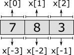
Besides obtaining a single element from a list, it is also possible to obtain a sub-range of the elements of a list, called a slice. Slicing also does not change the contents of the list. It results in a copy of a contiguous sub-sequence of the list. The result of a slice operation is again a list, even if the slice contains just one element, or no elements at all. Slicing requires two indices: the index of the first element of the sub-range (inclusive), and the index of the last element of the sub-range (exclusive). Both indices may be omitted. If the start index is omitted, it defaults to zero. If the end index is omitted it defaults to the length of the list. If the begin index is equal to or larger than the end index, the slice is empty. Similar to indexing, negative indices may be used, which are relative to the end of the list rather than the start of the list. Indices that are out of bounds saturate to those bounds. Some examples:
disc list int x = [7, 8, 3, 5, 9];

x[2:4]  //       [3, 5]    Slice that includes third and fourth elements.
x[2:7]  //       [3, 5, 9] Slice that excludes the first two elements.
x[1:]   //    [8, 3, 5, 9] Slice that excludes the first element.
x[:-1]  // [7, 8, 3, 5]    Slice that excludes the last element.
x[:]    // [7, 8, 3, 5, 9] Slice includes all elements (is equal to 'x').
The first slice takes the third (index 2) and fourth (index 3)
elements. The begin index (2) is thus included, the end index (4) is
not. The second slice starts at the same index, but extends to the sixth
element (index 7). Since there are only five elements, the index is
saturated (or clamped) to the end of the list. The results is that all but the
first two elements are included. The third slice excludes the first element
(index 0), by starting at index 1. It omits the end index, meaning that
the entire remainder of the list is kept, and only the first element is not
included. The fourth slice begins at the beginning of the list, as the begin
index is omitted. It continues until the last element of list, which it
excludes. It thus excludes a single element from the end of the list. The fifth
slice includes all elements, as both the begin and end index are omitted. The
slice is thus identical to the list in x. The following figure graphically
represents the slices:

Lists can be combined into new lists. They are essentially 'glued' together. This is called concatenation. This can also be used to add a single element to the front or back of the list. For instance:
[7, 8, 3] + [5, 9]   // [7, 8, 3, 5, 9]
[5] + [7, 8, 3]      // [5, 7, 8, 3]
[7, 8, 3] + [5]      // [7, 8, 3, 5]
Several other standard operators and functions are available to work with lists, including the following:
[1, 4, 2, 4, 5] - [2]           // [1, 4, 4, 5] (removal of elements)
[1, 4, 2, 4, 5] - [4]           // [1, 2, 4, 5]
[1, 4, 2, 4, 5] - [8]           // [1, 4, 2, 4, 5]
[1, 2, 3, 4, 5] - [6, 4, 2, 3]  // [1, 5]
[1, 4, 4, 1, 1] - [1, 4, 1]     // [4, 1]

[1, 8, 3] = [1, 3, 8]           // false (equality test)
6 in [1, 8, 3]                  // false (element test)
1 in [1, 8, 3]                  // true

empty([1, 2])                   // false (empty test)
size([1, 5, 3, 3])              // 4 (count elements)

del([7, 8, 9, 10], 2)           // [7, 8, 10] (removed value at index '2')
pop([1, 5, 3])                  // (1, [5, 3]) (first element and remainder)
Bounded lists and arrays
CIF can only represent lists (type list)
with at most 2,147,483,647 (= 231 - 1) elements. Using lists
with more elements results in the CIF model being invalid, and leads to runtime
errors. For instance, consider the following CIF specification:
automaton a:
  disc list int x;

  location:
    initial;
    edge do x := x + [1];
end
Each time the edge is taken, another element is added to list x. As soon
as an attempt is made to add the 2,147,483,648th element, a
runtime error occurs.
It is possible to explicitly restrict the number of elements that may be contained in a list:
disc list[3..7] int y; // List with at least 3 and at most 7 elements.
Variable y can only have lists as its value that have at least 3 and at
most 7 elements. Assigning a list with any other number of elements is not
allowed. Lists with size restrictions are called bounded lists. They can also
be called size restricted lists or ranged lists. The default value for
y is [0, 0, 0]. That is, the default value has the least amount of
elements that is allowed by the bounded list, and the default value (0) of
the element type (int).
Lists with a fixed length are called arrays:
disc list[5..5] int a;      // List with at least 5 and at most 5 elements.
disc list[5]    int b;      // Shorter but equivalent array notation.
By giving a bounded list the same lower and upper bound, the bounded list has a fixed number of elements, and can be called an array. Arrays also have a shorter and more convenient notation, where the number of elements is only given once. Both notations for arrays are equivalent.
Both bounded lists and arrays support the same operations as regular lists, and can be modified (assigned) the same way as regular lists, as long as their size restrictions are not violated.
Sets
A set is an unordered collection of values (called elements) of a same type. Each element value either exists in a set, or it does not exist in a set. Each element value is unique, as duplicate elements are silently discarded. Consider the following:
disc set int x1 = {3, 7, 8};
disc set int x2 = {8, 3, 7};        // Order irrelevant (same as 'x1').
disc set int x3 = {8, 3, 7, 3};     // Duplicates ignored (same as 'x2').
disc set int x4 = {};               // Empty set.
Variable x1 has a set of integers as its value. In this case, its initial
value is a literal set with three integer elements. As sets are unordered
collections of elements, {3, 7, 8} is the same set as {8, 3, 7}, and
thus variables x1 and x2 have the same initial values. Since elements
in a set are unique, set {8, 3, 7} is equal to the set {8, 3, 7, 3},
and thus variables x2 and x3 have the same initial values. For
readability, elements in a set are normally written in increasing order, for
example {3, 7, 8}. Variable x4 has an empty set as initial value, which
is also the default initial value for sets.
The union of two sets results in a set that contains the combined elements of
both sets. You can think of the resulting set containing the elements that are
in the one set or in the other set (or in both of them). Since sets never
contain duplicates, common elements are present only once in the resulting set:
{1, 2, 3} or {2, 3, 4}          // {1, 2, 3, 4}
{1, 2, 3} or {2, 3, 4}          // {1, 2, 4, 3}
Since sets are unordered, both answers are possible, and represent the same set. Since the order is irrelevant, there are 24 different ways to represent that same set. In the remainder of this lesson, we’ll use increasing order, for readability.
The intersection of two sets results in a set that contains the elements that
are present in both sets. You can think of the resulting set containing the
elements that are in the one set and in the other set. In other words, the
result contains the elements common to both sets:
{1, 2, 3} and {2, 3, 4}         // {2, 3}
{1, 2} and {3, 4}               // {} (no elements in common)
The difference of two sets results in a set that contains the elements of the first set that are not present in the second set. You can think of the resulting set containing the elements of the first set, with the elements of the second set subtracted or removed from it:
{1, 2, 3} - {2, 3, 4}           // {1}
{1, 2, 3} - {4, 5}              // {1, 2, 3}
{1, 2, 3} - {1, 2, 3, 4}        // {}
Several other standard operators and functions are available to work with sets, including the following:
{1, 8, 3} = {1, 3, 8}       // true (equality, ignores order of elements)

6 in {1, 8, 3}              // false (element test)
1 in {1, 8, 3}              // true

{1, 3} sub {1, 3}           // true (subset check)
{1, 3} sub {1, 3, 5}        // true
{1, 3} sub {1, 4}           // false
{1, 3} sub {1, 4, 5}        // false

empty({1, 2})               // false (empty test)
size({1, 5, 3, 3})          // 3 (count elements, duplicates ignored)
Dictionaries
A dictionary is an unordered collection of keys and associated values. A key with its associated value is called a key/value pair. Consider the following:
disc dict(string:int) age = {"eve":  32,
                             "john": 34,
                             "adam": 25};
Variable age has as value a dictionary consisting of pairs of strings
(the keys) and integers (the values). In this example, each string represents
a person’s name, and each integer represents the age of that person. Variable
age is initialized with a literal dictionary, containing three key/value
pairs. You can think of the dictionary as storing the information that eve
is 32 years old, or that the age of eve is 32.
As with sets, dictionaries are unordered. The order of the key/value pairs is
irrelevant, {"eve": 32, "adam": 25} is the same dictionary as
{"adam": 25, "eve": 32}. For readability, key/value pairs of dictionary
literals are normally written in increasing order of their keys.
{"adam": 25, "eve": 32} is thus preferred over {"eve": 32, "adam": 25},
as adam goes before eve in a phone book.
Dictionary literals are often written using multiple lines, to get two 'columns' for the keys and values, which can improve readability:
disc dict(string:int) age = {"eve": 32,
"john": 34,
"adam": 25};The default value for dictionary types, is an empty dictionary. The following two variables thus have the same initial value:
disc dict(string:int) x1 = {};  // Explicitly initialized as empty.
disc dict(string:int) x2;       // Implicitly initialized as empty.
Every key of a dictionary is unique, but they may be associated with the same value. For the above example with ages, the names (keys) are used to uniquely identify people, but multiple people may have the same age (values). It is not allowed to have the same key twice, in a dictionary literal, regardless of whether they map to the same value or to different values:
disc dict(int:int) x1 = {1: 2, 1: 2};  // Invalid due to duplicate key '1'.
disc dict(int:int) x2 = {1: 2, 1: 3};  // Invalid due to duplicate key '1'.
The values of a dictionary can be obtained by projection on that dictionary, using the keys:
disc dict(string:int) age = {"adam": 25, "eve": 32, "john": 34};
disc int i;

edge ... do i := age["adam"];   // 'i' becomes '25'
edge ... do i := age["eve"];    // 'i' becomes '32'
edge ... do i := age["carl"];   // error (there is no "carl" key)
Projection using a key that exists in the dictionary, results in the associated value. Projection using a key that does not exist in the dictionary, leads to a runtime error.
It is possible to modify single elements of a dictionary, as follows:
disc dict(string:int) age = {"adam": 25, "eve": 32, "john": 34};

edge ... do age["eve"] := 33;  // Changes eve's age.
edge ... do age["bob"] := 47;  // Adds a new key/value pair.
The age of eve is changed from 32 to 33. The age is thus replaced
by a new age. The age of bob is set to 47. Since there was no key/value
pair for that person in the dictionary, a new key/value pair is added. After
the updates of both edges, the value of variable age is
{"adam": 25, "bob": 47, "eve": 33, "john": 34}.
Several other standard operators and functions are available to work with dictionaries, including the following:
{"a": 1, "b": 2} = {"b": 2, "a": 1}     // true (equality check)
{"a": 1, "b": 2} = {"a": 1, "b": 3}     // false

"a" in {"a": 1, "b": 2}                 // true (key existence check)
"c" in {"a": 1, "b": 2}                 // false

{"a": 1, "b": 2} + {"b": 3, "c": 4}     // {"a": 1, "b": 3, "c": 4} (add/overwrite pairs)

{"a": 1, "b": 2} - {"b": 3, "c": 4}     // {"a": 1} (removal based on keys)
{"a": 1, "b": 2} - {"b", "c"}           // {"a": 1}
{"a": 1, "b": 2} - ["b", "c"]           // {"a": 1}

empty({"a": 1, "b": 2})                 // false (empty check)
size({"a": 1, "b": 2})                  // 2 (count pairs)
Combining values
Values of different types can usually be arbitrarily combined. For instance, consider the following example:
disc dict(int;tuple(real pos, weight)) boxes = {1: (0.0, 2.5),
                                                2: (3.0, 1.7),
                                                3: (4.0, 3.9};
Variable boxes stores data about multiple boxes, in a dictionary with
unique identification numbers (1, 2, and 3) used as keys. For each
box, the position (pos) and weight are stored as a tuple. Initially,
there are three boxes. The first box has identification number 1,
position 0.0, and weight 2.5. The second box has identification number
2, position 3.0, and weight 1.7. Also consider the following
example, where the data of that variable is manipulated:
edge ... do boxes[1][weight] := 3.5;
edge ... do boxes[2][pos] := boxes[2][pos] + 1;
edge ... do boxes[4] := (1.0, 0.8);
The first edge changes the weight of the box 1 (the box with
identification number 1), from 2.5 to 3.5. The second edge
increases the position (pos) of box 2 from 3.0 to 4.0. The
third edge adds data for a new box with identification number 4.
Scalable solutions and reuse (1/2)
Constants
Through the use of constants, fixed values can be given a name. Using constants, it is easy to change certain fixed values. If the constant is used consistently throughout the model, the value needs to be changed only in one place. Constants can thus make it easier to keep the model consistent.
Consider the following CIF specification:
const int STEP = 2;
const int TARGET = 100;

automaton movement:
  disc int position = 0;
  event move;

  location:
    initial;
    edge move when position < TARGET do position := position + STEP;
end
In this example, the movement automaton keeps track of the position of
an object. The object starts at position 0. It can move until it
reaches its target position. The target position is 100. Rather than using
position < 100 as guard, the value 100 is stored in a constant named
TARGET. The constant can then be used instead the value 100. Similarly,
the step size of the object is stored in a constant named STEP.
Constants have a name, which by contention is usually written using upper case
letters. Using a constant instead of a fixed value makes it more clear what
that value represents. For instance, by using position < TARGET rather than
position < 100, the intention of the guard condition is more clear. Using a
constant can thus enhance readability.
Another benefit of constants, is that they can be used multiple times in the same model:
const int STEP = 2;
const int TARGET = 100;

automaton movement:
  disc int position = 0;
  event forward, backward;

  location:
    initial;
    edge forward  when position < TARGET do position := position + STEP;
    edge backward when position > 0      do position := position - STEP;
end
In this modified example it is possible for the object to perform forward
as well as backward movements. The step size is the same for both
movements, making it possible to use the STEP constant in the updates of
both edges. Since a constant is used, the speed of both movements can be
changed by changing the value of the constant. Without using a constant, the
speed would have to be changed separately for each edge.
Constants are not limited to integer values. Consider the following example, where a more complex value is used:
enum ProductType = A, B, C;
const dict(ProductType:real) DURATION = {A: 3.5, B: 5.7, C: 0.8};
This example declares a ProductType enumeration, with three different
product types: A, B, and C. The DURATION constant indicates
for each product type, how long it takes to produce a product of that type.
Products of type A can be produced in 3.5 hours, products of type B
in 5.7 hours, etc. To get the production duration of products of type C,
expression DURATION[C] can be
used. For more information, see the lessons on
enumerations and
dictionaries.
Algebraic variables
Consider a conveyor belt with a product on it:

The product starts at the left side, at position 0. There is a sensor that
can detect the product between positions 13 and 14. The product exits
the conveyor at position 18. The following CIF specification models the
conveyor, product, and sensor:
automaton conveyor:
  disc real position = 0.0;
  event move;

  const real width = 6;
  alg bool sensor = position + width >= 13 and position <= 14;

  location:
    initial;
    edge move when position < 18 do position := position + 0.1;
end
The conveyor automaton models the conveyor, with a product on it. The
product is modeled by means of the position of the left side of the
product, relative to the left side of the conveyor. As the conveyor starts to
move, the product moves as well, and its position on the conveyor is
updated. The product moves in steps of 0.1.
The width of the product is 6. The sensor is on whenever
the product, which spans from position to position + width, is within
the sensor range, which spans from 13 to 14. An algebraic variable
named sensor is used here, to represent the value of the sensor.
An algebraic variable is a variable whose value is determined by its
definition. For the sensor variable, its value is determined from a
calculation involving variable position and constant width. Unlike
discrete variables, algebraic variables can not be assigned a new value. The
value of algebraic variable sensor changes automatically as the value of
discrete variable position changes. The value of algebraic variable
sensor is true whenever the product is over the sensor, and it is
false otherwise.
If we had modeled the value of the sensor as a discrete variable, we would have
had to update the variable for every edge where the value of variable
position is updated. In this example, that is only one edge. However, if
the variable would have been updated on multiple edges, the sensor value would
also have to be updated for all those edges. Furthermore, when adding
another edge that updates the position variable, the edge needs to be
adapted to also update the sensor discrete variable, which can easily be
forgotten. Using an algebraic variable, the value computation needs to be
specified only once, and no changes to its value are needed, as the value
always remains consistent with its definition.
Algebraic variables can be used to give an expression (computations) a name, similar to how constants can be used to give fixed values a name. The benefits of using an algebraic variable are similar to the benefits of using constants. Both can be used to improve readability, and to make it easier to consistently change the model.
Algebraic variables can also be used as an abstraction. Consider the following extension of the specification:
automaton light:
  event turn_on, turn_off;

  location off:
    initial;
    edge turn_on  when     conveyor.sensor goto on;

  location on:
    edge turn_off when not conveyor.sensor goto off;
end
The idea is to have a light turn on when a product is detected by the sensor,
and have it turn off when the sensor no longer detects the product. The
algebraic variable sensor is used in the guard conditions of the light
automaton, to determine when the light should be turned on or off.
In the example, the light automaton only uses the sensor variable from
automaton conveyor. It does not matter how the value of that variable is
defined. Currently, it is defined in terms of variable position and
constant width. However, if the conveyor automaton were modeled
differently, the expression that defines the value of the algebraic variable
could be changed, without the need to change the use of the variable in
automaton light.
Algebraic variables and equations
Consider the following CIF specification:
automaton car:
  event start, stop, breakdown, start_repair, repaired;

  alg bool can_drive = idle or moving;

  location idle:
    initial;
    edge start goto moving;

  location moving:
    edge stop goto idle;
    edge breakdown goto broken;

  location broken:
    edge start_repair goto repairing;

  location repairing:
    edge repaired goto idle;
end
The car is initially idle. Once you start driving, the car is
moving. Once you stop driving, the car is idle again. While
moving it is possible for a breakdown to occur, meaning the car is
broken. Once a mechanic starts the repair (start_repair), the mechanic
is repairing the car. Once it is repaired, the car is idle, and you
can start driving it again, etc.
Algebraic variable can_drive indicates whether you can currently drive the
car. As the value calculation indicates, the car can be driven whenever it is
idle or moving. That is, it can’t be driven if the car is broken
or a mechanic is repairing it.
In the example above, the value of the algebraic variable is defined with the declaration, as was already explained in the lesson that introduced algebraic variables. However, it also possible to specify the value separately, using an equation:
automaton car:
  event start, stop, breakdown, start_repair, repaired;

  alg bool can_drive;

  equation can_drive = idle or moving;

  // Locations omitted for brevity.
end
This allows for separation of variable declarations and equations. Both
variants have the same algebraic variable with the same value. An equation of
an algebraic variable must be placed in the same component as where the
algebraic variable is declared. In the example above, the equation for
algebraic variable can_drive must be placed in automaton car, as that
is where the algebraic variable is declared.
For algebraic variables declared in automata, it is also possible to specify the value using an equation per location of the automaton:
automaton car:
  event start, stop, breakdown, start_repair, repaired;

  alg bool can_drive;

  location idle:
    initial;
    equation can_drive = true;

    edge start goto moving;

  location moving:
    equation can_drive = true;

    edge stop goto idle;
    edge breakdown goto broken;

  location broken:
    equation can_drive = false;

    edge start_repair goto repairing;

  location repairing:
    equation can_drive = false;

    edge repaired goto idle;
end
Every algebraic variable must have a unique value in every situation. Algebraic variables must thus have a value with their declaration, a single equation in the same component, or an equation in every location of the automaton. For every algebraic variable, one of the three variants must be chosen. It is allowed to choose a different variant for different algebraic variables, but it is not allowed to use multiple variants for the same algebraic variable.
Which variant fits best for a specific algebraic variable, depends on the situation. One of the benefits of using an equation per location, is that the equations are checked for completeness. If you add a new location, you must add an equation to that location as well, as otherwise the model is invalid (incomplete). This means you can’t forget to specify the value of the algebraic variable for that new location. If you use a value with the declaration or a single equation in the component, you might forget to update the value for the changes you made to the automaton.
Type declarations
Consider this slightly modified version of an example from the lesson on constants:
enum ProductType = A, B, C;

const dict(ProductType:real) M1_DURATION = {A: 3.5, B: 5.7, C: 0.8};
const dict(ProductType:real) M2_DURATION = {A: 1.8, B: 4.2, C: 3.9};
This example declares a ProductType enumeration, with three different
product types: A, B, and C. The M1_DURATION constant indicates
for each product type, how long it takes to produce a product of that type,
on machine 1. Products of type A can be produced in 3.5 hours, products of
type B in 5.7 hours, etc. Constant M2_DURATION is similar, but for
machine 2.
The type of both constants is the same. To avoid having to repeat complex types in multiple places, a type declaration can be used:
enum ProductType = A, B, C;
type Durations = dict(ProductType:real)

const Durations M1_DURATION = {A: 3.5, B: 5.7, C: 0.8};
const Durations M2_DURATION = {A: 1.8, B: 4.2, C: 3.9};
A type declaration with name Durations is introduced, and Durations can
then be used wherever a type is expected, instead of
dict(ProductType:real). In the example above, Durations is used as
type of the two constants. The original specification and the one with the
type declaration have the same constants, with effectively the same type. That
is, in both specification the value of constant M1_DURATION is a
dictionary with three key/value pairs.
Type declarations can be used to give a type a name, similar to how constants can be used to give fixed values a name, and algebraic variables can be used to give computations a name. The benefits are also similar, as type declarations can be used to make specifications more concise, to increase readability, and to make it easier to consistently change types throughout the specification.
Time
Timing
So far, the tutorial has only used discrete event models as examples, which are all untimed. This lesson introduces the concept of timing.
In CIF, time starts at zero (0.0). Time can progress continuously. That is,
after one unit of time has passed, the model time is 1.0. After an
additional one and a half time units have passed, the model time is 2.5,
etc. By default, one time unit corresponds to one second. However, you can
decide to use another unit, and tools such as the simulator can be configured
to speed up or slow down the simulation accordingly.
Variable time
A variable named time is always available in every specification. The
variable holds the current absolute model time as its value, and can be used
throughout the model. Initially, time and thus the value of variable time
start at zero (0.0). As time progresses, the value of variable time is
automatically updated to ensure it properly represents the current time of the
system.
In this lesson, absolute time will be used. In most models, it is easier to use relative time. This can be achieved with continuous variables, discussed in the next lesson.
Timed guards
Consider the following CIF specification:
event push, release;

automaton user:
  location start1:
    initial;
    edge push    when time >= 1.5 goto stop1;

  location stop1:
    edge release when time >= 2.3 goto start2;

  location start2:
    edge push    when time >= 2.4 goto stop2;

  location stop2:
    edge release when time >= 7.6 goto done;

  location done;
end
The push and release events represent pushing and releasing of a button
respectively. The actual behavior of the button itself is omitted. The
specification does model the behavior of a user. Initially, the user
is in location start1, and no time has passed. The edge with the push
event is not yet enabled, as the guard is not satisfied. As soon as one and a
half time units have passed, the guard condition becomes satisfied, and the
push event becomes enabled. This edge models that the user starts to push
the button after 1.5 time units. The user then waits for another 0.8
(2.3 - 1.5) time units, before releasing the button (stop pushing it).
After waiting another 0.1 (2.4 - 2.3) time unit, the user pushes
the button again. Finally, after waiting 5.2 (7.6 - 2.4) time
units, the user releases the button one last time. In the done location,
the push and release events are never enabled (no edges for those
events), and thus the user never pushes or releases the button again. No other
events are enabled, so time keeps progressing forever, without any events
happening.
Time transitions
The state space of the above specification is:

The states are labeled with the names of the current locations of automaton
user and the current values of variable time. The transitions labeled
with event names are event transitions. The other transitions are
time transitions, which are labeled with the duration of the time
transitions, i.e. the number of time units that passes. At the end of the
state space, a time transition of infinite duration is shown, to indicate that
time can progress forever.
The current locations of automata can not change as time passes as the result of taking a time transition. The only way for the current locations to change, is as the result of taking an edge as part of an event transition.
Urgency
By default, all events in CIF are urgent. Events being urgent means that edges are taken as soon as possible. In other words, event transitions take priority over time transitions. Time can only progress if no event transitions are possible. For further details on urgency, see the future urgency lesson.
Numeric time
In the above example, guard time >= 1.5 is used. You might wonder why the
guard is not time = 1.5, as the intention is that user pushes the button
after exactly 1.5 time units, and not after 1.6 or 1.7 time units.
The main reason is that the simulator uses finite
precision in its numeric calculations to find the moment in time that the edge
becomes enabled. The answer also has finite precision. It is often not exactly
at 1.5 time units, but is slightly after it, say at time
1.50000000000001. If you use time = 1.5 as guard instead of
time >= 1.5, the simulator will most likely
miss the change in enabledness of
the edge, and will never enable the event.
Continuous variables
In the lesson that introduced timing, variable
time was used. Variable time uses absolute model time, i.e.
the total amount of time that has passed since the start of the simulation.
It is usually easier to use relative model time, i.e. a certain amount of time
passes after a certain event. This is where continuous variables are ideal.
A continuous variable is a variable that changes value automatically, as time
progresses. Consider the following CIF specification:
automaton machine:
  event start, finished;
  cont t = 0 der 1;

  location idle:
    initial;
    edge start do t := 0 goto producing;

  location producing:
    edge finished when t >= 3 goto idle;
end
This specification models a machine that is initially idle. The machine
can start to produce a product. After a while, it is done producing.
Due to having finished the product, it becomes idle again, until it is
starts to product the next product.
Continuous variable t is declared to initially have value 0. Its
derivative is 1, meaning that every unit of time that passes, the value
of t increases by 1. Every time the start event happens, the value
of continuous variable t is reset to 0 using an assignment. As a result
of this reset, t will be 0 when the automaton enters the producing
location. The edge for the finished event indicates that the event can only
happen when t >= 3 holds. This condition will hold after three time units.
This means that automaton machine remains in the producing location for
three time units, before going to the idle location. It will thus always
take three units after entering the producing location, before the guard
becomes enabled, and the finished event can take place. The state space is
as follows:

The states are labeled with the first letters of the names of the current
locations of automaton machine and the current values of variables time
and t.
Continuous variables always have real values.
Similar to discrete variables, if their initial value is not specified, it is
0.0:
cont t der 1; // Initial value is 0.0.The derivative of a continuous variable can be used as a variable as well. The
derivative of continuous variable t is t'. A derivative is read only;
it can not be assigned. Similar to algebraic variables, it is always equal to
its definition. In the case of variable t, its derivative is always 1.
The values of variables time, t, and t' as time progresses are:

Continuous variables and equations
Consider the following CIF specification:
automaton person:
  event turn;
  cont t = 0 der 1;

  location:
    initial;
    edge turn when t > 10 do t := 0.0;
end
This specification models a person walking back and forth. Every time that
the person has walked 10 time units, (s)he will turn around, walking
in the other direction.
In the example above, the derivative of the continuous variable is defined with the declaration, as was already explained in the lesson that introduced continuous variables. However, it also possible to specify the derivative separately, using an equation:
automaton person:
  event turn;
  cont t = 0;         // Declaration specifies only the initial value.

  equation t' = 1;    // Derivative specified using separate equation.

  location:
    initial;
    edge turn when t > 10 do t := 0.0;
end
This allows for separation of variable declarations and equations. Both
variants have the same continuous variable with the same derivative. An
equation of a derivative of a continuous variable must be placed in the same
component as where the continuous variable is declared. In the example above,
the equation for t' must be placed in automaton person, as that is
where t is declared.
We could extend this specification to keep track of the direction that the person is moving:
automaton person:
  event turn;
  cont t = 0 der 1;

  location away:
    initial;
    edge turn when t > 10 do t := 0.0 goto back;

  location back:
    edge turn when t > 10 do t := 0.0 goto away;
end
For continuous variables declared in automata, it is also possible to specify the derivative using an equation per location of the automaton. This allows us to keep track of the exact position of the person:
automaton person:
  event turn;
  cont pos = 0;

  location away:
    initial;
    equation pos' = 1;
    edge turn when pos > 10 goto back;

  location back:
    equation pos' = -2;
    edge turn when pos < 0 goto away;
end
Here, the continuous variable t has been renamed to pos, to make it
more clear that it indicates the position of the person. As long as the
person is moving away, the derivative of pos is 1, and the
person moves away, one place every time unit. When the person reaches
position 10, the position is not reset to zero. Instead, only the location
is changed to the back location. In that location, the derivative of
pos is -2. This means that every time unit, the position decreases
by 2. That is, the person back to the original position, but at twice the
speed. The values of variables time, pos, and pos' as time
progresses are:

As with algebraic variables, every continuous variable must have a unique derivative in every situation. Continuous variables must thus have a derivative with their declaration, a single equation in the same component, or an equation in every location of the automaton. For every continuous variable, one of the three variants must be chosen. It is allowed to choose a different variant for different continuous variables, but it is not allowed to use multiple variants for the same continuous variable.
Equations
Consider the following non-linear system:

Variable V models the water volume of a tank. The water volume of the tank
changes based on the incoming flow of water Qi and outgoing flow of water
Qo. The tank can be modeled using the following CIF specification:
cont V = 5 der Qi - Qo;
alg real Qi = 1;
alg real Qo = sqrt(V);
Initially, the tank is filled with 5 liters of water. The incoming flow is
constant at 1 liter per second. The outgoing flow increases as the water
volume of the tank increases.
By separating the declarations of the three variables from their equations, the specification becomes more readable:
cont V = 5;
alg real Qi;
alg real Qo;

equation V' = Qi - Qo;
equation Qi = 1;
equation Qo = sqrt(V);
The values of the variables as time passes are shown in the following figure:
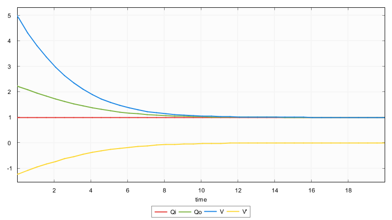
Variables overview
CIF features different kinds of variables, that have different functionality. Each is better suited for a particular purpose. The following table gives an overview:
| Kind of variable | Can be assigned | Can change as time progresses |
|---|---|---|
yes |
no |
|
no |
yes |
|
yes |
yes |
|
no |
yes |
Discrete variables can only change value when given an explicit new value by means of an assignment. They don’t change automatically as time progresses.
Algebraic variables can’t be assigned. Instead, their values depend on their declarations or equation(s). If the computations that result in their values depend on a variable that can change value as time progresses, then so can the values of the algebraic variables. Algebraic variables are used as named shorthand notations for computations, for readability, reuse, consistency, and abstraction.
Continuous variables automatically change value as time progresses, as specified by their derivatives. They can also be assigned new values, from which they then automatically change again, based on the current values of their derivatives.
The derivatives of the continuous variables can be seen as variables themselves. Their values depend on their declaration or equation(s). If the computations that result in their values depend on a variable that can change value as time progresses, then so can the values of the derivatives.
Urgency
In CIF, urgency indicates whether or not time may progress. CIF has three forms of urgency: event urgency, location urgency, and edge urgency. Edge urgency should be avoided, and is not explained here.
Event urgency
By default, all events in CIF are urgent. Events being urgent means that edges are taken as soon as possible. In other words, event transitions take priority over time transitions. Time can only progress if no event transitions are possible. It is not possible to make events non-urgent in a CIF model, but specific tools may allow making events non-urgent.
Location urgency
Consider the following CIF specification:
automaton use_case:
  location first:
    initial;
    edge tau goto second;

  location second:
    edge tau goto done;

  location done;
end
This automaton represents a use case, which goes from one location to the next. The state space is:

The states are labeled with the names of the current locations of automaton
use_case and the current values of variable time. At the end of the use
case, no events are possible, and thus time can progress infinitely. To force
that in location done no time can progress, the location can be made
urgent:
automaton use_case:
  location first:
    initial;
    edge tau goto second;

  location second:
    edge tau goto done;

  location done:
    urgent; // Location is now urgent.
end
The resulting state space is:

Deadlock and livelock
This lesson explains the concepts of deadlock and livelock.
Deadlock
If no event transitions are possible, and also no time transitions are possible (time may not progress), then no transitions are possible. This is called deadlock. No behavior is possible, or will ever become possible. As an example, consider the following CIF specification:
automaton use_case:
  location wait3:
    initial;
    urgent;
    edge tau when time > 3 goto done;

  location done;
end
Location wait3 is the initial location. Initially, time is zero. Time
can not progress, as the location is urgent.
Since the guard of the edge also does not hold, event tau is also not
possible. No transitions are possible, and the specification is in deadlock.
Livelock
As long as an event is possible, no time may pass. If by mistake always an event is possible, this prevents all passage of time. Consider the following CIF specification:
automaton car:
  event increase, decrease, arrived;
  disc real speed = 0;
  cont pos der speed;

  location underway:
    initial;
    edge increase when speed < 100 do speed := speed + 1;
    edge decrease when speed > 0   do speed := speed - 1;
    edge arrived  when pos = 850 goto done;

  location done;
end
This specification models a car that can increase and decrease its
speed, so that it is at least 0 and at most 100. It keeps track of its
position (continuous variable pos) that increases more quickly as the speed
increases. When position 850 is reached, the car has arrived and is
done.
The car will be increasing and decreasing it speed, using the increase and
decrease events. As always at least one of them is enabled at any moment,
time can never progress, and pos remains zero. This effect is called
livelock. While behavior is still possible, the model does not truly progress
with useful behavior. The model gets 'stuck' repeating one or a few events.
Channel communication
Channels
Consider the following figure of a producer and two consumers, where rectangles represent entities and the arrows represent the data that is communicated:
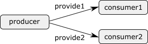
The producer creates products, identified by a unique identification number. Each product produced by the producer, is provided either to the first or to the second consumer. Consider the following CIF specification:
event provide1, provide2;

automaton producer:
  disc int nr = 0;

  location:
    initial;
    edge provide1, provide2 do nr := nr + 1;
end

automaton consumer1:
  disc int nr = -1;

  location:
    initial;
    edge provide1 do nr := producer.nr;
end

automaton consumer2:
  disc int nr = -1;

  location:
    initial;
    edge provide2 do nr := producer.nr;
end
The producer keeps track of the identification number (variable nr) of
the current product, and provides products to either the first consumer
(event provide1) or the second consumer (provide2). Both consumers
have an identification number of their current product as well (variable
nr in the consumer automata). Initially, the consumers don’t have a
product, as indicated by value -1. When a consumer gets a new product, it
looks up the identification number of the product at the producer, and stores
it locally. The producer then moves on to the next product, by increasing its
current identification number.
We can identify two problems in this model.
The first problem is that we need two events in order for the producer to
provide products to either the one consumer or the other consumer. If we
used only one event, both consumers would need to use that event, have the
event in their alphabet, and would thus have
to simultaneously participate in the
synchronization. A consequence of
having an event per consumer, is that the producer automaton has both
events on its edge. Adding a third consumer entails having to add another
event, as well as having to modify the edge of the producer automaton. This
is not a nice scalable solution.
The second problem is that the consumer refers directly to the nr variable
of the producer automaton. This introduces a very tight coupling between
the producer and the consumers. It exposes the nr variable of the
producer to the consumers, making it more difficult to change the producer
without changing the consumers.
Both these problems can be solved by using channels. Channels are a special form of events, that can be used to communicate or transmit data from a sender to a receiver. In our example, data that is communicated are the identification numbers of the products, the producer is the sender, and the consumers are the receivers.
Channels require one or more potential senders, and one or more potential receivers. Automata cannot be both sender and receiver for a single channel. They may however be a sender for one channel, and a receiver for another channel. For every transition, exactly one of the senders and exactly one of the receivers participate. The sender sends a value, and the receiver receives that value. This type of communication is often called channel communication or point-to-point communication, as the data is communicated from one point (the sender) to another point (the receiver).
Multiple automata that synchronize over the same event perform a transition together. Similarly, a sender and receiver that together perform a channel communication, perform a transition together. In both cases, all automata involved take their respective edges synchronously (simultaneously).
Channels are ideally suited for modeling product flows, or more generally the movement of physical entities through a system. Physical objects usually don’t duplicate themselves or spontaneously stop to exist. This fits nicely with channels, where data is communicated or passed along from exactly one sender to one receiver. In our example, product produced by the producer are physically provided to one of the consumers.
The following CIF specification models the above example using channels:
event int provide;

automaton producer:
  disc int nr = 0;

  location:
    initial;
    edge provide!nr do nr := nr + 1;
end

automaton consumer1:
  disc int nr = -1;

  location:
    initial;
    edge provide? do nr := ?;
end

automaton consumer2:
  disc int nr = -1;

  location:
    initial;
    edge provide? do nr := ?;
end
The provide1 and provide2 events have been replaced by a single
channel named provide. Channels are declared similar to events, but have a
data type that indicates the type
of values that are communicated
over the channel. In this case integers are
communicated.
The producer now uses the channel on its edge, instead of the two events.
The exclamation mark (!) after the channel name means that the producer
is sending over the channel. After the exclamation mark, the value that the
producer sends is given. In this case, the producer sends the identification
number of its current product.
The edges of the consumers have been modified as well. The channel is used
with a question mark (?) after the channel name, indicating that the
consumers receive over the channel. The received value, which is available as
the ? variable in the update, is directly assigned to the nr variable
of the consumer.
By using channels, we no longer need multiple events, and the producer does not
need to be modified if another consumer is added. This makes the model scalable
to varying amount of consumers. Furthermore, the consumers now use the ?
variable to obtain the received value, and no longer need direct access to the
variables of the producer. This makes it easier to modify the producer
without having to also modify the consumers.
To conclude this lesson, we’ll extend the example with a second producer:
event int provide;

automaton producer1:
  disc int nr = 0;

  location:
    initial;
    edge provide!nr do nr := nr + 1;
end

automaton producer2:
  disc int nr = 0;

  location:
    initial;
    edge provide!nr do nr := nr + 1;
end

automaton consumer1:
  disc int nr = -1;

  location:
    initial;
    edge provide? do nr := ?;
end

automaton consumer2:
  disc int nr = -1;

  location:
    initial;
    edge provide? do nr := ?;
end
The producer automaton has been renamed to producer1, and a
producer2 has been added. Both producers independently produce products
and provide them to the consumers. Both consumers can receive products from
either producer. At all times, four transitions are possible:
producer1 communicates with consumer1, producer1 communicates with
consumer2, producer2 communicates with consumer1, or producer2
communicates with consumer2.
Dataless channels
Besides channels that communicate data, it is also possible to use dataless
channels. A channel that does not communicate any data, is declared with the
void type. Dataless channels are also called void channels. When using
dataless channels, the sender does not provide a value to send over the
channel. Also, the receiver cannot use the received value (variable ?)
since no data is communicated.
Dataless channels are used in the same situations as 'normal' channels, for instance when physical product flow is modeled. If products don’t have an identification number, and can not be distinguished based on color or some other property, all products are essentially equal. It is then sufficient to communicate that a product is being 'transferred'. No further data is needed. While it is possible to communicate dummy values, dataless channels provide a better solution in such cases.
Consider again the producer/consumer example from the previous lesson, with one producer and two consumers, but without identification numbers for the products:
event void provide;

automaton producer:
  location:
    initial;
    edge provide!;
end

automaton consumer1:
  location:
    initial;
    edge provide?;
end

automaton consumer2:
  location:
    initial;
    edge provide?;
end
The producer still produces products and provides them to either the first
or the second consumer.
Combining channel communication with event synchronization
Consider again the producer/consumer example with two producers and two consumers, from a previous lesson:
event int provide;

automaton producer1:
  disc int nr = 0;

  location:
    initial;
    edge provide!nr do nr := nr + 1;
end

automaton producer2:
  disc int nr = 0;

  location:
    initial;
    edge provide!nr do nr := nr + 1;
end

automaton consumer1:
  disc int nr = -1;

  location:
    initial;
    edge provide? do nr := ?;
end

automaton consumer2:
  disc int nr = -1;

  location:
    initial;
    edge provide? do nr := ?;
end
Now assume we want to restrict communication to allow at most five products in total to be provided to the consumers. We could adapt both producers, as follows:
automaton producer1:
  disc int nr = 0;

  location:
    initial;
    edge provide!nr when nr + producer2.nr < 5 do nr := nr + 1;
end

automaton producer2:
  disc int nr = 0;

  location:
    initial;
    edge provide!nr when producer1.nr + nr < 5  do nr := nr + 1;
end
Each producer gets an additional guard condition whether it may provide a product to one of the consumers. If the total number of products provided by both providers does not exceed five, they may still provide a product. Having to adapt both producers is less than ideal.
As an alternative solution, we can add an additional automaton, instead of adapting the producers:
automaton controller:
  disc int cnt = 0;

  location:
    initial;
    edge provide when cnt < 5 do cnt := cnt + 1;
end
This controller automaton (together with the original producer automata)
keeps track of the number of products provided to consumers, by counting them
in variable cnt. It only allows the provide event when less than five
products have been provided. If five or more products have been provided, it
disables the provide event.
In the controller automaton, the provide channel is used as an event
rather than a channel. When one of the producers and one of the consumers
together perform a channel communication, the controller automaton that has
the provide event in its alphabet, must
synchronize with it. This allows the controller to impose additional
restrictions on the channel communication, allowing or forbidding it in
certain cases. The controller is added as a separate process, which
improves scalability.
In general, every automaton may either send over a channel, receive over a channel, or synchronize with a channel. An automaton may not take on more than one of these roles, for a single event. It may however send over one channel, receive over another channel, and synchronize with yet another one.
Every event transition for a channel requires exactly one automaton that participates as sender, and exactly one automaton that participates as receiver. Furthermore, all automata that have the channel in their alphabet, must additionally participate as well, by synchronizing together with the sender and receiver. Automata that send or receive over a channel, do not have that channel in their alphabet. Only automata that synchronize with an event or channel have that event or channel in their alphabet.
Automata that synchronize over a channel can be used to further restrict the allowed channel communications, as shown in the above example. It is however also possible for the additional synchronizing automata to monitor (observe) the channel communication.
Functions
Functions
Functions can be used to compute values from other values. CIF has many
built-in functions, called standard library functions. An example is the
size function, which takes a list and
returns the number of elements of the list. Another example is the abs
function, which takes an integer or
real number and computes the absolute value of
that number.
While many built-in functions are available, they may not always suffice. User-defined functions can be added to CIF models, to allow custom computations needed by the model. By putting the calculation in a user-defined function, the calculation can be used in several places, allowing for reuse. Furthermore, functions allow for more complex computations than would otherwise be possible.
CIF features two kinds of user-defined functions: internal ones and external ones. Internal user-defined functions are fully defined within the CIF model. External user-defined functions declare only a header which indicates the existence of the function, while the actual implementation is obtained from an external source. The lessons of this category only explain internal user-defined functions. The language reference documentation gives more information on external user-defined functions.
Internal user-defined functions
The most commonly used kind of user-defined functions are the internal user-defined functions. Consider the following CIF specification:
func real mean(list real vs):
  int length = size(vs);
  int index = 0;
  real sum = 0;

  while index < length:
    sum := sum + vs[index];
    index := index + 1;
  end
  return sum / length;
end
This specification defines a function (keyword func) named mean. After
the name of the function, between the parentheses, the parameters are listed.
The parameters are the input values, which the function can use to compute its
result. In this example, the function takes a
list of real
values as its only parameter. Parameter name vs can be used in the body of
the function to refer to this input value. Just after the func keyword, the
type of the result of the
computation is specified. In this case, the function results in a
real typed value. The mean function takes a
list of integer values and produces a single real value as result.
In the body of the function, local variables can be declared. The mean
function declares three variables: length, index, and sum. Local
variables of functions are very similar to
discrete variables. The main
difference is that they are
declared without the disc keyword. In the example, length is set to the
number of elements in list vs. Variables index and sum are both
initialized to 0.
After the local variables (if any), the statements of the body are given. The
statements implement the algorithm, the actual computation of the function.
Statements are executed one after another, in the order they are given. In the
mean function, the while statement is executed before the return
statement. The mean function first calculates the sum of the input values,
and then returns the mean value. The details of the statements are discussed
in the next lesson.
A function can be called (or applied) on concrete input values, to obtain the computation result for those specific input values. For instance, consider the following extension to the above CIF specification:
alg real m = mean([1.5, 3.2, 7.9, 15.8]);

automaton a:
  disc real x;

  location:
    initial;
    edge do x := 2 * mean([0.4, 1.5, 6.8]);
end
Algebraic variable m is given the value that results from calling function
mean on a single argument, a list with four values. Each argument of a
function call must match with the corresponding parameter of the function being
called. In this case, the list of four real values matches with the vs
parameter of the mean function, which has type list real. Variable
m becomes 7.1, as the mean of those four values is 7.1
((1.5 + 3.2 + 7.9 + 15.8) / 4).
The edge in automaton a assigns a value to variable x. The mean of a
list of three values is calculated, and multiplied by two, to obtain the new
value of x. The mean of 0.4, 1.5, and 6.8 is
(0.4 + 1.5 + 6.8) / 3, which is 2.9. Variable x gets 5.8
(2.9 * 2) as its new value.
Function mean is called in two places in the example, showing reuse of
calculations.
Functions in CIF are mathematical functions. That is, the result of a function
is the same for the same input values, and functions have no side effects.
Functions can not directly access variables outside their body. For example,
they cannot access discrete, continuous, and algebraic variables. They can also
not use variable time. To use the values of those variables in a function,
they have to to be passed in through parameters.
Function statements
This lesson explains the different statements that can be used in internal user-defined functions:
Assignment statement
Assignments in functions are very similar to assignments to discrete variables. For instance:
x := x + 1;Besides local variables, it also allowed to assign new values to the parameters. Changes to parameters only have effect inside the function itself.
For multi-assignments, the outer parentheses are not needed:
// Multi-assignment on an edge.
edge do (x, y) := (1, 2);

// Multi-assignment in a function.
x, y := 1, 2;
If statement
It is possible to perform different calculations under different circumstances. Consider the following function:
func int signum(real x):
  if x > 0:
    return 1;
  elif x < 0:
    return -1;
  else
    return 0;
  end
end
This signum function takes a real number x and returns its
sign.
The if statement
is used to detect the different situations, and to return the correct result
in each of those situations.
Return statement
The execution of a function ends when a return statement is encountered.
The value following the return statement is the result of the entire
function. Consider again the return statement from the mean function
from the previous lesson:
return sum / length;In this case, the sum of the input values is divided by the number of input
elements (variable length) to obtain the mean of the input values. The mean
of the input values is the result of the function.
While statement
The while statements allows for repeated execution of the statements in its
body, as long as the condition of the while loop holds. Consider again the
mean function from the
previous lesson:
func real mean(list real vs):
  int length = size(vs);
  int index = 0;
  real sum = 0;

  while index < length:
    sum := sum + vs[index];
    index := index + 1;
  end
  return sum / length;
end
The mean function processes each of its input values, using a while
loop. As long as the condition (index < length) holds, the body of the
while is executed over an over. The body consists of two assignments. The
first assignment obtains an input value (vs[index]) and adds it to the
sum. The second statement increases the index, to proceed with the next
input value. After the two assignments have been executed, the condition of the
while is evaluated again. If the condition still holds, the two assignments
are executed again, etc. When the condition no longer holds, the while
statement is done, and execution proceeds with the next statement, the
return statement.
Break statement
A break statement 'jumps out' of a while statement, continuing with the
first statement after the while. Consider the following CIF specification:
// Get the first 'n' values from 'xs' that are not 'bad'.
func list int first_n(list int xs; int n; int bad):
  int index = 0;
  int x;
  list int result = [];

  while index < size(xs):
    x := xs[index];
    if x != bad:
      result := result + [x];
    end
    if size(result) = n:
      break;
    end
    index := index + 1;
  end
  return result;
end

// The value of 'y' is [1, 5, 3].
alg list int y = first_n([1, 2, 5, 3, 4, 1, 3], 3, 2);
The first_n function takes a list of integer numbers xs, and returns a
list result with the first n numbers from xs that are not bad.
A while loop is used to process each of the numbers in list xs. The
current number is stored in variable x. If the current number is not the
same as bad, it is added to the result. If the result then contains
n values, the break statement is used to break out of the while
loop and continue execution at the first statement after the while loop,
which is the return statement. If less than n values are in the result,
index is incremented to ensure the next number of the list is processed in
the next iteration of the while loop. The return statement at the end
of the function is used to return the result list, which contains at most
n values.
Continue statement
A continue statement 'jumps over' the remaining statements in the body
of a while statement, and continues with the next iteration of that
while statement. Consider the following CIF specification:
// Get the values from 'xs' that are greater than 5.
func list int filter_gt5(list int xs):
  int index = 0;
  int x;
  list int result = [];

  while index < size(xs):
    x := xs[index];
    index := index + 1;
    if x <= 5:
      continue;
    end
    result := result + [x];
  end
  return result;
end

// The value of 'y' is [8, 7, 6].
alg list int y = filter_gt5([1, 8, 5, 7, 4, 6, 3]);
The filter_gt5 function takes a list of integer numbers, and returns a
filtered list that only contains those integer number that are greater than 5.
A while loop is used to process each of the numbers in list xs. The
current number is stored in variable x, and index is incremented to
ensure the next number of the list is processed in the next iteration of the
while loop. If the current number is not greater than 5, the remaining
statements in the body of the while are skipped, meaning x is not
added to the result. The while loop then continues with the next
iteration, for the next number in xs. If the current number (x) is
greater than 5, execution continues after the if statement, and the number
is added to the result. After all numbers in the list have been processed,
the filtered result list is returned to the caller of the function.
Functions as values
Functions can be used as values. By treating them as data, they can be stored in variables, and passed to other functions. This lesson shows one example of how that can be useful.
Consider the following list of numbers:
alg list real nrs = [0.5, 1.3, 0.1, 2.7, 1.4];Now assume we wanted to sort these numbers both in increasing and in decreasing order, using a single sorting function:
alg list real inc = sort(nrs, cmp_inc); // [0.1, 0.5, 1.3, 1.4, 2.7]
alg list real dec = sort(nrs, cmp_dec); // [2.7, 1.4, 1.3, 0.5, 0.1]
Variable inc contains the same numbers as nrs, but sorted in increasing
order, while dec contains them in decreasing order. We use the same
sort function in both cases, but with different comparison functions:
func bool cmp_inc(real a, b):
  return a <= b;
end

func bool cmp_dec(real a, b):
  return a >= b;
end
Function cmp_inc takes two real numbers and returns true only if the
first number is smaller than the second one (a and b are in increasing
order). Function cmp_dec has the same parameters, but returns true only
if the first number is larger than the second one (a and b are in
decreasing order). The sort function is defined as follows:
func list real sort(list real xs; func bool (real, real) cmp):
  int i = 1, j;
  real x;

  while i < size(xs):
    j := i;
    while j > 0 and not cmp(xs[j-1], xs[j]):
      // swap x[j-1] and x[j]
      x := xs[j-1];
      xs[j-1] := xs[j];
      xs[j] := x;
      j := j - 1;
    end
    i := i + 1;
  end
  return xs;
end
The sort function has two parameters. The first parameter is xs, which
contains the values to sort. The second parameter is cmp, the compare
function to use to determine whether two numbers are correctly ordered. The
cmp parameter has type func bool (real, real), which means that a
function that has two real parameters and a boolean return value is required.
The cmp_inc and cmp_dec functions satisfy these requirements, and can
be used as second argument when the function is called to determine the values
of algebraic variables inc and dec.
The sort function implements a standard
insertion sort
algorithm. The
cmp parameter is used in the sort function to compare two consecutive
values in xs, and swap them if they are not correctly ordered.
The cmp parameter of the sort function has a function type, allowing
compare functions to be passed to the sort function, as data. This allows
the sort function to sort lists of numbers in different orders, depending
on the compare function that is provided.
Scalable solutions and reuse (2/2)
Automaton definition/instantiation
Parts of a system that are nearly identical, are often modeled as nearly identical automata. Having to specify them multiple times can be burdensome. It can also hinder scalability, as changes to one of them usually need to be applied to the others as well. Consider again the producer/consumer example from the lesson that introduced channels:
event int provide;

automaton producer:
  disc int nr = 0;

  location:
    initial;
    edge provide!nr do nr := nr + 1;
end

automaton consumer1:
  disc int nr = -1;

  location:
    initial;
    edge provide? do nr := ?;
end

automaton consumer2:
  disc int nr = -1;

  location:
    initial;
    edge provide? do nr := ?;
end
The producer provides products either to the first consumer or to the second
consumer. The consumers are modeled using identical automata. Only the names of
the consumer1 and consumer2 automata differ. Ideally, we would have a
sort of consumer template, and use that template twice, once for each of the
actual consumers. This can be achieved in CIF using an automaton definition
(the template) and two automaton instantiations (the uses of the template):
event int provide;

automaton producer:
  disc int nr = 0;

  location:
    initial;
    edge provide!nr do nr := nr + 1;
end

automaton def Consumer():
  disc int nr = -1;

  location:
    initial;
    edge provide? do nr := ?;
end

consumer1: Consumer();
consumer2: Consumer();
The Consumer automaton definition is identical to the original consumers,
except that it is an automaton definition rather than an automaton. An
automaton definition can be identified by the def keyword between the
automaton keyword and the name of the automaton definition, as well as by
the parentheses after its name. As a convention, names of automaton definitions
start with an upper case letter (Consumer rather than consumer).
An automaton definition by itself is not an automaton. The instantiations of
the automaton definition (consumer1 and consumer2) however, are
automata. Before the colon (:), the name of the instantiation is given.
This name is also the name of the actual automaton. After the colon, the name
of the automaton definition that is instantiated is given.
Using an automaton definition, the above example models the behavior of a
consumer only once. Adding a third consumer is as easy as adding another
automaton instantiation, which takes only one line of code
(consumer3: Consumer();). Changing the behavior of all consumers only
requires changes to the common automaton definition. Automaton
definition/instantiation allows for scalability and reuse, and also improves
maintainability.
Automaton definition/instantiation can be eliminated, by replacing all
automaton instantiations by the automaton definitions that they instantiate,
and changing the automaton definition header (automaton def Consumer():) by
an automaton header (automaton consumer1:). If we do that for the example
above, we obtain the original specification from the beginning of this lesson.
The two specifications are functionally equivalent. Automaton instantiation
consumer1 is also often referred to as automaton consumer1, when there
is no confusion.
Parametrized automaton definitions
In the previous lesson, automaton definition/instantiation was used to obtain two identical automata, while only having to specify their behavior once. What we have seen so far, is enough for exactly identical automata, but not for nearly identical automata. Consider the following two nearly identical consumers:
automaton consumer1:
  disc list int buffer = [];

  location:
    initial;
    edge provide? when size(buffer) < 2 do buffer := buffer + [?];
end

automaton consumer2:
  disc list int buffer = [];

  location:
    initial;
    edge provide? when size(buffer) < 3 do buffer := buffer + [?];
end
The consumers can accept products that the producer provides (channel
provide). They store the identification numbers of those products in a
buffer. The two consumers are identical except for the number of products
that they can accept: the first consumer can accept two products, the second
producer can accept three products. We can still use automaton definition and
instantiation to model the consumer only once, but we need to parametrize the
automaton definition:
automaton def Consumer(alg int capacity):
  disc list int buffer = [];

  location:
    initial;
    edge provide? when size(buffer) < capacity do buffer := buffer + [?];
end

consumer1: Consumer(2);
consumer2: Consumer(3);
The Consumer automaton definition now has a parameter named capacity
that indicates how many identification numbers can be stored in its buffer.
The automaton instantiations consumer1 and consumer2 provide an
argument (2 and 3 respectively) to match the parameter of Consumer.
That is, the instantiations indicate their capacity. Using parameters, the
Consumer automaton definition models the behavior of both automata
consumer1 and consumer2, even though they have different capacities.
The details of the different kind of parameters of automaton definitions are explained in the next lesson.
Automaton definition parameters
In the previous lesson, an automaton definition with parameter was used. The parameter was an algebraic parameter, which is only one of the different kinds of automaton definition parameters. This lesson explains each of them:
This lesson also explains how to use multiple parameters.
Algebraic parameters
An algebraic parameter is similar to an algebraic variable. Arbitrary values or expressions of matching type can be provided as arguments in automaton instantiations. For instance, consider the following partial CIF specification:
event int accept, provide;

automaton def Buffer(alg int capacity):
  disc list int buf = [];

  location:
    initial;
    edge accept?        when size(buf) < capacity do buf := buf + [?];
    edge provide!buf[0] when size(buf) > 0        do buf := buf[1:];
end

buffer1: Buffer(5);
Automaton definition Buffer has an algebraic parameter that indicates the
capacity of the buffer. The buffer can accept something when it has not
yet reached its capacity. It can provide something when the buffer is not
empty. Automaton instantiation buffer1 has value 5 as its parameter.
Value 5 is an integer number, which matches the integer type (int) of
the capacity parameter.
Algebraic parameters can be used inside an automaton definition, wherever a value is expected, e.g. in guards, updates, initial values of discrete variables, and invariants. The expression that is provided by the instantiation is essentially filled in wherever the parameter is used. The above is equivalent to:
event int accept, provide;

automaton buffer1:
  disc list int buf = [];

  location:
    initial;
    edge accept?        when size(buf) < 5 do buf := buf + [?];
    edge provide!buf[0] when size(buf) > 0 do buf := buf[1:];
end
Event parameters
Event parameters allow different instantiations to synchronize with different events or to communicate over different channels. For instance, consider the following partial CIF specification:
event int generate, pass_along, exit;

automaton def Buffer(event int accept, provide):
  disc int buffer;

  location accepting:
    initial;
    edge accept? do buffer := ? goto providing;

  location providing:
    edge provide!buffer goto accepting;
end

buffer1: Buffer(generate, pass_along);
buffer2: Buffer(pass_along, exit);
Automaton definition Buffer is parametrized with two channels, one to
accept a product into the one place buffer, and one to provide it to
some other part of the system. The first buffer (buffer1) accepts products
via the generate channel, and provides products via the pass_along
channel. The second buffer (buffer2) accepts products via the
pass_along channel, and provides products via the exit channel. The
first buffer uses the pass_along channel as its provide channel
parameter, and the second buffer uses that same pass_along channel as its
accept channel parameter. The first buffer thus provides its items to the
second buffer.
Event and channel parameters can be used inside an automaton definition, wherever an event or channel is expected, e.g. on edges and in alphabets if explicitly specified. The event or channel that is provided by the instantiation is essentially filled in wherever the parameter is used. The above is equivalent to:
event int generate, pass_along, exit;

automaton buffer1:
  disc int buffer;

  location accepting:
    initial;
    edge generate? do buffer := ? goto providing;

  location providing:
    edge pass_along!buffer goto accepting;
end

automaton buffer2:
  disc int buffer;

  location accepting:
    initial;
    edge pass_along? do buffer := ? goto providing;

  location providing:
    edge exit!buffer goto accepting;
end
Channel parameter usage restrictions
If an event parameter is actually a channel (it has a data type), it may also
be called a channel parameter. By default, a channel parameter can be used to
send, receive, or synchronize. However, it is also possible to restrict the
allowed usages. By putting certain event usage restriction flags after the name
of the channel parameter, only those usages are allowed. The available flags
are ! to allow sending, ? to allow receiving, and ~ to allow
synchronizing. Duplicate flags are not allowed, the ! should be before the
? flag, and the ! and ? flags should be before the ~ flag.
By restricting the usages, you can immediately see how a channel parameter is used within the automaton definition, as only the usages indicates by the parameter are allowed. It serves as sort of documentation of the intention of the channel parameter. This is much simpler than finding the actual usages of the parameter in the automaton. However, note that the parameter indicates the allowed usages, and doesn’t guarantee that the event/parameter is actually used at all.
Another benefit of restricting the usages, is that it makes it possible to spot
mistakes. You might for instance use a channel parameter on an edge (e.g.
edge e), but forget to include the send part (e.g. edge e!1). If the
parameter only allows sending, the accidental synchronization (edge e) is
reported as an invalid use. Without the usage checking, you might not encounter
the problem until for instance simulation, where it is much more difficult to
find the cause.
For the example above, we have the following header of the Buffer
definition:
automaton def Buffer(event int accept, provide):We can change this as follows:
automaton def Buffer(event int accept?, provide!):This makes it clearer that the accept channel is used to receive a
product into the buffer, and the provide channel is used send a product
from the buffer.
Location parameters
An earlier lesson explained how a location can be used as a variable. Using location parameters, automaton definitions can be supplied with different locations. For instance, consider the following CIF specification:
automaton def Machine(location other_processing):
  location heat_up:
    initial;
    edge when not other_processing goto processing;

  location processing:
    edge tau goto cool_down;

  location cool_down:
    edge tau goto heat_up;
end

machine1: Machine(machine2.processing);
machine2: Machine(machine1.processing);
Automaton definition Machine represents a machine that can heat up, process
something, cool down, and repeat that forever. The system consists of two of
those machines. The machines can not start processing if the other machine is
already processing. That is, the machines perform
mutually exclusive
processing. If the first machine is in its processing location, the other
can’t also be processing (in its own processing location). To prevent a
machine from starting to process if the other machine is already processing,
each machine needs to know whether the other is already processing. Therefore,
automaton definition Machine is parametrized with a location parameter
other_processing, that indicates whether the other machine is currently
processing (in its processing location). This parameter is used as a guard
that determines whether a transition from location heat_up to location
processing is allowed. Automaton instantiation machine1 provides the
first machine with the processing location of the second machine, by
using machine2.processing as its instantiation argument.
Location parameters can be used inside an automaton definition, wherever a boolean value is expected, e.g. in guards. The location that is provided by the instantiation is essentially filled in wherever the parameter is used. The above is equivalent to:
automaton machine1:
  location heat_up:
    initial;
    edge when not machine2.processing goto processing;

  location processing:
    edge tau goto cool_down;

  location cool_down:
    edge tau goto heat_up;
end

automaton machine2:
  location heat_up:
    initial;
    edge when not machine1.processing goto processing;

  location processing:
    edge tau goto cool_down;

  location cool_down:
    edge tau goto heat_up;
end
Automaton parameters
When multiple declarations (variables, locations, etc) from one automaton are to be supplied as parameters to another automaton, it is also possible to supply the entire automaton as a parameter, but only if the provided automaton is an instantiation of an automaton definition. Consider for instance the following CIF specification:
automaton def Sensor():
  event go_on, go_off;

  location off:
    initial;
    edge go_on goto on;

  location on:
    edge go_off goto off;
end

sensor1: Sensor();
sensor2: Sensor();

automaton def Actuator(Sensor sensor):
  event turn_on, turn_off;

  location off:
    initial;
    edge turn_on  when sensor.on  goto on;

  location on:
    edge turn_off when sensor.off goto off;
end

actuator1: Actuator(sensor1);
Automaton definition Sensor models a sensor that can go on an off. Both
sensor1 and sensor2 are actual sensors. Automaton definition
Actuator models an actuator that can be turned on if a sensor is on, and be
turned off if that same sensor is off. The actuator1 automaton is provided
sensor1 as sensor. If sensor1 goes on, actuator1 is turned on, and
if sensor1 goes off, actuator1 is turned off. sensor2 going on or
off has no effect on actuator1.
Automaton parameters can be used inside an automaton definition, to refer to declarations inside the automaton supplied for the automaton parameter. The automaton that is provided by the instantiation is essentially filled in wherever the parameter is used. The above is equivalent to:
automaton sensor1:
  event go_on, go_off;

  location off:
    initial;
    edge go_on goto on:

  location on:
    edge go_off goto off:
end

automaton sensor2:
  event go_on, go_off;

  location off:
    initial;
    edge go_on goto on:

  location on:
    edge go_off goto off:
end

automaton actuator1:
  event turn_on, turn_off;

  location off:
    initial;
    edge turn_on  when sensor1.on  goto on;

  location on:
    edge turn_off when sensor1.off goto off;
end
Multiple parameters
It is possible to use multiple parameters of the same kind, as well as different kinds of parameters:
automaton def X(event a, b; alg real c; event d):
  ...
end

event z;

x: X(z, z, 3 * 5, z);
Automaton definition X has four parameters: a, b, c, and d.
Since a and b are both event parameters, a comma (,) is used to
make sure the event keyword does not need to be repeated for parameter
b. Algebraic parameter d is of a different kind, and is therefore
separated using a semicolon (;).
Automaton instantiation x instantiates X with the event z (for the
first, second, and fourth parameters), and value 15.0 (3 * 5, for the third
parameter).
Groups
For large CIF specifications with many automata, it can be beneficial to add more structure to the specification. For this purpose, CIF has groups. Groups are named collections of automata and other declarations. For instance, consider the following CIF specification:
group factory:
  group hall1:
    automaton machine1:
      ...
    end

    automaton machine2:
      ...
    end
  end

  group hall2:
    automaton machine1:
      ...
    end

    automaton machine2:
      ...
    end
  end
end
This specifications features four automata that model the behavior of machines.
The details of the actual automata are omitted, as they are irrelevant for this
lesson. All four machines are in the same factory, but they are divided into
two halls. This physical subdivision is expressed in the CIF specification
using groups named factory, hall1, and hall2. While in this case
the subdivision into a hierarchical specification structure is based on the
physical subdivision of the actual system, the modeler is free to base the
specification structure on other criteria.
Consider also the following partial CIF specification:
group configuration:
  const int  MAX_PRODUCTS        = 1500;
  const real MAX_PRODUCTION_TIME = 3.7;
  const real ARRIVAL_RATE        = 28.6;
end
The configuration group is used to group together several configuration
values, modeled by constants. By grouping these constants together, it is more
clear that they together are the configuration settings of the system, and that
they belong together.
Finally, consider the following CIF specification, based on the non-linear system from the lesson on equations.
group tank:
  cont V = 5;
  alg real Qi;
  alg real Qo;

  equation V' = Qi - Qo;
  equation Qi = 1;
  equation Qo = sqrt(V);
end
By grouping the declarations and their equations together, it is becomes clear
that together they model a tank. This is especially useful if other parts
of the specification model something different.
Group definitions
Similar to how automaton definitions can be used for reuse of automata, group definitions can be used for reuse of groups:
automaton def Machine():
  location:
    initial;
  ...
end

group def Hall():
  machine1: Machine();
  machine2: Machine();
end

group def Factory():
  hall1: Hall();
  hall2: Hall();
end

factory1: Factory();
Automaton definition Machine models a machine, but most of the details are
omitted here, as they are not relevant for this lesson. Group definition
Hall models that each hall has two machines. Similarly, group definition
Factory models that each factory has two halls.
Automata and groups are both components in CIF. Automaton definitions and group definitions can together be called component definitions. If we eliminate all component definitions and their instantiations, by replacing instantiations by their definitions, we get the following CIF specification:
group factory1:
  group hall1:
    automaton machine1:
      location:
        initial;
      ...
    end

    automaton machine2:
      location:
        initial;
      ...
    end
  end

  group hall2:
    automaton machine1:
      location:
        initial;
      ...
    end

    automaton machine2:
      location:
        initial;
      ...
    end
  end
end
Group definitions may be parametrized using the same kinds of parameters as automaton definitions.
Imports
For large systems, having to model the entire system in a single CIF file can
lead to long CIF specifications. Being able to split that single CIF file into
multiple CIF files can help. Consider the following two CIF specifications in
CIF files producer.cif and consumer.cif respectively:
// producer.cif

event provide;

automaton producer:
  location:
    initial;
    edge provide;
end
// consumer.cif
import "producer.cif";
automaton consumer:
location:
initial;
edge provide;
endThe two CIF specifications together form a simplified producer/consumer system.
The producer.cif file declares the provide event and the producer
automaton. The producer can provide a product.
The consumer.cif file declares the consumer automaton, that can accept
products provided by a producer. The provide event is not declared in that
CIF specification. However, the producer.cif file is imported, which does
declare that event. By importing another CIF specification, all declarations
from that imported CIF specification (producer.cif in the example) become
available in the importing CIF specification, i.e. in the specification that
does the import (consumer.cif in the example).
The result of the import in consumer.cif is:
event provide;

automaton producer:
  location:
    initial;
    edge provide;
end

automaton consumer:
  location:
    initial;
    edge provide;
end
You can think of an import as being replaced by the content of the imported
file. The producer.cif file contains only its own content, while the
consumer.cif file contains the contents of both files, due to the use of
the import.
If one CIF specification is merged into another CIF specification, the names of
the declarations in both CIF specifications must be different. It is not
allowed to have declarations with the same name in multiple CIF specifications.
For instance, in the example above, if the provide event were declared in
both CIF specifications, the imports would be invalid. Exceptions to this rule
are discussed in one of the next lessons, which explains the relation between
imports and groups.
Imports and libraries
Using imports, it is possible to make
libraries that can be used by multiple CIF specifications. For instance,
consider the following CIF specification in file math.cif:
// math.cif

func int inc(int x):
  return x + 1;
end
This CIF specification declares a single function inc that takes an integer
number and returns that number incremented by one. Now also consider the
following CIF specification in file counter.cif:
// counter.cif

import "math.cif";

automaton counter:
  disc int count = 0;

  location:
    initial;
    edge tau do count := inc(count);
end
By importing the math.cif file, the counter automaton can use the
inc function. Other CIF files could similarly import the math.cif file,
essentially turning math.cif into a library.
It is possible to make a function library, consisting of commonly used functions, a constant library, with commonly used constants, or an automaton definition library, with automaton definitions. As libraries are just CIF files, they can contain anything as long as they are valid CIF files. Essentially, every CIF file that is imported in more than one other CIF file can be considered a library.
The import as used above, only works if both CIF files are in the same directory. Library files however, are often placed in a different directory. Consider the same two CIF files, but organized into directories (or folders) as follows:

Directory system contains a sub-directories named libraries, which
contains the math.cif library. The system directory also contains the
counter.cif file. The import in the counter.cif file needs to be
adapted to refer to the math.cif file in the libraries directory:
// counter.cif

import "libraries/math.cif";

automaton counter:
  disc int count = 0;

  location:
    initial;
    edge tau do count := inc(count);
end
Imports and groups
Large systems can be hierarchically modeled using groups. When using imports, two specifications may not have declarations with the same name. Groups however, are the exception to this rule. Consider a factory with two machines, each consisting of two parts. We can model this using five files, one for each of the parts of the machines, and one for the factory as a whole. The following CIF specifications show the contents of the five CIF files, where the comment at the first line indicates which file it is:
// p1.cif

group machine1:
  automaton part1:
    location idle:
      initial;
      edge tau goto running;

    location running:
      edge tau goto idle;
  end
end
// p2.cif
group machine1:
automaton part2:
location idle:
initial;
edge tau goto running;
location running:
edge tau goto idle;
end
end// p3.cif
group machine2:
automaton part1:
location idle:
initial;
edge tau goto running;
location running:
edge tau goto idle;
end
end// p4.cif
group machine2:
automaton part2:
location idle:
initial;
edge tau goto running;
location running:
edge tau goto idle;
end
end// factory.cif
import "p1.cif";
import "p2.cif";
import "p3.cif";
import "p4.cif";The four CIF specifications for the machine parts differ only in their group
and automaton names. Their implementations are kept identical for simplicity.
The factory.cif file imports all four part specifications, which together
form the full factory. The effect of the imports in factory.cif is the
following:
group machine1:
  automaton part1:
    location idle:
      initial;
      edge tau goto running;

    location running:
      edge tau goto idle;
  end

  automaton part2:
    location idle:
      initial;
      edge tau goto running;

    location running:
      edge tau goto idle;
  end
end

group machine2:
  automaton part1:
    location idle:
      initial;
      edge tau goto running;

    location running:
      edge tau goto idle;
  end

  automaton part2:
    location idle:
      initial;
      edge tau goto running;

    location running:
      edge tau goto idle;
  end
end
For groups with the same name, the contents of the groups is merged together.
That is, automaton part1 in the machine1 group from one CIF file, and
the automaton part2 in that same machine1 group from another CIF file,
end up in a single machine1 group after eliminating the imports.
In general, contents of groups with the same name are merged into a single
group. This works also for groups in groups, groups in groups in groups, etc.
If two CIF files that are imported both contain a group a and in both CIF
files those groups contain a group b, then the contents of both a
groups are merged, and also the contents of both b groups are merged. It is
not allowed for different CIF files to have declarations with the same name in
the same group. It is allowed to have declarations with the same name in
different groups. The file itself (the top level) can be considered a group as
well.
Namespaces
When using imports and groups to model large hierarchical systems, it is a common pattern to have groups around the entire specification:
group factory:
  group machine1:
    group part1:
      automaton sensor1:
        ...
      end

      automaton actuator1:
        ...
      end
    end
  end
end
The groups around the entire specification lead to additional indentation. As this is a common pattern, the CIF language provides namespaces to reduce the impact of large numbers of top level groups:
namespace factory.machine1.part1;

automaton sensor1:
  ...
end

automaton actuator1:
  ...
end
The factory.machine1.part1 namespace has exactly the same effect as the
original three groups. Both specifications can thus be considered identical.
Input variables
Input variables can be used to model that some data exists, without specifying the value or how or when the value changes. Input variables are used in cases where the CIF model is to be connected something else that provides the values.
Hardware example
The CIF model may for instance be a controller that is to be connected to a piece of physical hardware. The input variables then model sensors, for which the behavior is not modeled in the CIF model. As an example, consider the following CIF specification:
input bool sensor;

automaton controller:
  cont t der 1;
  alg bool actuator = on;

  location off:
    initial;
    edge when sensor do t := 0 goto waiting;

  location waiting:
    edge when not sensor goto off;
    edge when t > 1.5 goto on;

  location on:
    edge when not sensor goto off;
end
Input variable sensor models a digital sensor. When the sensor is on, the
variable has value true and when the sensor is off, the variable has value
false. When the sensor is on and when it is off is not known, and thus not
modeled in the CIF specification.
The controller waits (in location off) for the sensor to go on, and
then resets continuous variable t to start measuring 1.5 time units
(in location waiting). If that much time has passed, it goes to location
on. If the sensor goes off then, or while it is waiting, it goes back to
location off. Thus, the controller is only on if the sensor goes
on, 1.5 time units have passed, and the sensor remains on.
The actuator algebraic variable models that an actuator is only on if the
controller is in its on location. The actuator is then on if the sensor
is one, and 1.5 time units have passed. The actuator is always turned off
when the sensor is off.
Without a physical hardware system, the CIF specification is incomplete, as the value of the sensor is not known. The input variable acts as a placeholder for the actual sensor. If the CIF specification were to be coupled to a physical hardware system with a sensor and an actuator, the CIF model would then control the actuator based on the sensor values.
Co-simulation example
A CIF specification could model a part of a system, while another part of that same system is modeled in another system or language, such as Simulink. Consider for instance a tank filled with water. Water flows out of the tank constantly. By opening a value, water also flows in to the tank. Consider the following CIF specification:
input real level;

automaton valve:
  disc bool open = true;

  location:
    initial;
    edge when     open and level >= 10 do open := false;
    edge when not open and level <=  2 do open := true;
end
The water level is modeled as an input variable, meaning it is obtained
from the Simulink model. The CIF specification models the valve, and the
controller that opens and closes the value, based on the water level. It keeps
the level between 2 and 10.
The CIF model obtains the water level from Simulink by means of input variable
level. It also provides the open variable of the valve automaton to
Simulink. This variable can be used in Simulink to model how the water level
changes over time.
Without the Simulink model, the CIF specification is incomplete, as the water level is not known. The input variable acts as a placeholder for the actual water level. If the CIF specification were to be coupled to a Simulink model that models the water level, the CIF specification would control the valve based on the water level.
CIF models example
Input variables can also be used to couple CIF models. Consider again the above water level controller example. It models the valve and controls the valve, but does not model the water level. The following CIF specification could be used to model the water level:
cont level der if valve.open: 1 else -1 end;

group valve:
  input bool open;
end
Continuous variable level models the water level. The water level increases
(derivative 1) if the valve is open, and decreases (derivative -1)
otherwise. The open variable from the valve is used, but this variable
is an input variable, and the value is not known in this specification. Input
variable open acts as a placeholder for a value, and group valve acts
as a placeholder for automaton valve.
The two CIF specifications both model a part of the system. One specification models the water level, and has a placeholder for the variable that indicates whether the valve is open. The other specification models the valve and controls it, but has a placeholder for the water level. If we couple the two CIF specifications, they provide each other with actual variables for each others input variables.
The two specifications can be coupled or merged together:
cont level = 0.0 der if valve.open: 1 else -1 end;

automaton valve:
  disc bool open = true;

  location:
    initial;
    edge when     open and level >= 10 do open := false;
    edge when not open and level <=  2 do open := true;
end
Using input variables to couple CIF specifications is somewhat similar to using imports to split a CIF specification over multiple files. There are however important differences.
The first difference is that when using imports, one CIF specification is coupled to another CIF specification. The coupling is hard-coded in the CIF specification, and can not be changed without changing the import. When using input variables and merging, it is possible to couple a CIF specification to a second CIF specification, and later couple it with a third, different specification instead. The decision about which models to merge can thus be postponed, and does not require changes to any of the CIF specifications.
Another difference is that with imports it is not allowed to have declarations with the same name in different CIF specifications (except for groups), while with the merger this is allowed in many situations. See the documentation of the CIF merger tool for further details on what can be merged using that tool.
Stochastics
Stochastics
For many things in the world, the behavior is not the same every time. An example is a coin toss, where the result can be either heads or tails. Tossing a coin exhibits randomness. It is possible to model the different variants in a CIF model without specifying the likelihood of each of the outcomes. This approach was used in the lesson on non-determinism.
It is however also possible to explicitly specify the likelihood of each of the outcomes in the CIF model, using a stochastic distribution (also called probability distribution). A stochastic distribution describes how likely the different outcomes are. There are many different stochastic distributions. The Bernoulli distribution for instance, can be used to model things with two potential outcomes, such as a coin toss.
Consider the following CIF specification:
automaton coin_toss:
  disc dist bool d = bernoulli(0.5);
  disc bool outcome;

  location toss:
    initial;
    edge do (outcome, d) := sample d goto result;

  location result:
    edge when     outcome goto heads;
    edge when not outcome goto tails;

  location heads:
    edge tau goto toss;

  location tails:
    edge tau goto toss;
end
Variable d holds a stochastic distribution that produces
boolean values (true or false), as
indicated by its dist bool
type. In this case it holds a
Bernoulli distribution, with a probability of 0.5 (or chance of 50%) for
true, and thus also the same probability/chance for false (the only
other possible outcome).
The bernoulli function is used to create a Bernoulli distribution with the
proper parameter (probability of 0.5 for true). Different distributions
have different parameters. See the language reference documentation for further
details. Distribution functions, such as the bernoulli function can be used
to create distributions with specific parameters, and may only be used to
initialize discrete variables.
Initially, the automaton is in its toss location, where the coin can be
tossed. The edge uses the sample operator to get a sample from the
bernoulli distribution. Each time the distribution is sampled, the outcome
is either a true value or a false value. As we used a probability of
0.5 for both outcomes, half of the times true will be the outcome,
and the other half of the times false will be the outcome, if we were to
sample infinitely many times.
Sampling does not only result in the outcome, but also the distribution
itself. This is further explained in one of the next lessons, which explains
pseudo-randomness.
The result of sampling is stored in the outcome variable. In the result
location, the sampling result is used to make a decision to go to either the
heads location (true outcome) or the tails location (false
outcome). From there, it is possible to go back to the toss location, to
proceed with the next coin toss.
Discrete, continuous, and constant distributions
CIF features over a dozen different stochastic distributions. These distributions can be categorized into three categories: discrete, continuous, and constant distributions. Discrete distributions can result in only a limited number of possible values. Examples include tossing a coin (heads and tails) and throwing a dice (six possible outcomes). Continuous distributions can result in all values from a certain range. Examples include the time it takes for a machine to produce a single product (positive amount of time), and the purity of produced medicine (0% to 100%). Constant distributions are discrete distributions that always result in the same sampled value. They are useful during the development of a model, or for debugging. The remainder of this lesson further explains these three categories, and illustrates them using some examples.
Discrete distributions
Discrete distributions can result in only a limited number of possible values. The lesson that introduced stochastics used the discrete Bernoulli distribution to model tossing of a coin, which can result in either heads or tails.
Throwing a dice can result in six possible outcomes: 1, 2, 3, 4, 5, and 6. For a fair dice, each of the outcomes is equally likely, with chance 1/6. This can be modeled using a discrete uniform distribution:
automaton dice:
  disc dist int d = uniform(1, 7);
  disc int result;
  disc list int results = [];

  location throw:
    initial;
    edge do (result, d) := sample d goto add;

  location add:
    edge do results := results + [result] goto throw;
end
The uniform function is used to create a uniform integer distribution that
produces integer samples from the range
[1..7) (inclusive on the left side, exclusive on the right side). Each sample
is stored in result and added to the results. If we were to simulate
this model forever, the results list would contain equal amounts of each of
the six values.
Continuous distributions
Continuous distributions return a value from a continuous range. An example is the weight of pennies. This could for instance be approximated using a continuous normal distribution with a mean of 2.46 grams and a variance of 0.0004 grams:
automaton pennies:
  disc dist int d = normal(2.46, 0.0004);

  location:
    initial;
    edge do (weight, d) := sample d;
end
The normal function is used to create a normal distribution with a mean of
2.46 and a variance of 0.0004. The sampled weight is stored in the
weight variable each time the distribution is sampled. The probability of
the different weights as a result of the used normal distribution is depicted
in the following figure:

Constant distributions
When developing a model with stochastic behavior, it can be hard to validate whether the model behaves correctly, since the stochastic results make it difficult to predict the outcome of experiments. As a result, errors in the model may not be noticed, as they hide in the noise of the stochastic results. One solution is to first make a model without stochastic behavior, validate that model, and then extend the model with stochastic sampling. Extending the model with stochastic behavior is however an invasive change that may introduce new errors. These errors can again be hard to find due to the difficulties to predict the outcome of an experiment. The constant distributions aim to narrow the gap by reducing the amount of changes that need to be done after validation.
With constant distributions, a stochastic model with sampling of distributions is developed, but the stochastic behavior is eliminated by temporarily using constant distributions. The model performs stochastic sampling of values, but with predictable outcome, and thus with predictable experimental results, making validation easier. After validating the model, the constant distributions are replaced with the distributions that fit the mean value and variation pattern of the modeled system, giving a model with stochastic behavior. Changing the used distributions is however much less invasive, making it less likely to introduce new errors at this stage in the development of the model.
Constant distributions always produce the same sampled value. Consider the following CIF specification:
automaton dice:
  disc dist int d = constant(3); // Constant distribution.
  disc int result;
  disc list int results = [];

  location throw:
    initial;
    edge do (result, d) := sample d goto add;

  location add:
    edge do results := results + [result] goto throw;
end
This model is identical to the dice model one used earlier in this lesson,
except for distribution variable d, which now holds a constant distribution
that only produces value 3 when sampled.
Pseudo-randomness
So far, the lessons on stochastics used the mathematical notion of stochastic distribution to describe how to model stochastic behavior. Simulating a model with stochastic behavior using a computer is however not stochastic at all. Computer systems are deterministic machines, and have no notion of varying results.
Pseudorandom number generator and seed
A pseudorandom number generator is used to create stochastic results instead. It starts with an initial seed, an integer number. From this seed, a function creates a stream of 'random' values. When looking at the values there does not seem to be any pattern. It is not truly random however. Using the same seed again gives exactly the same stream of numbers. This is the reason to call the function a pseudorandom number generator, as a true random number generator would never produce the exact same stream of numbers.
Simulation and initial seed
A sample of a distribution uses one or more numbers from the stream to compute its value. The value of the initial seed thus decides the value of all samples drawn in the simulation. By default, a different seed is used each time you run a simulation, leading to different results each time. You can also explicitly state what seed you want to use when simulating a model. See the Stochastic distributions and seeds page of the simulator for information on how to supply a custom seed for simulation.
While doing a stochastic simulation study, performing several experiments with the same initial seed invalidates the results, as it is equivalent to copying the outcome of a single experiment a number of times. On the other hand, when looking for the cause of a bug in the model, performing the exact same experiment is useful as outcomes of previous experiments should match exactly.
Sampling and tuple results
The seed determines the next sampled value. Whenever a distribution is sampled, the seed changes to the one that follows in the stream of random numbers generated by the pseudorandom number generator. This ensures that the next time the distribution is sampled, it results in a different sampled value.
In CIF, the seed is stored with the distribution and its parameters. Therefore, sampling does not only result in the sampled value, it also results in an updated distribution, with the same parameters, but a different seed value.
Consider the following CIF specification:
automaton coin_toss:
  disc dist bool d = bernoulli(0.5);
  disc bool outcome;

  location:
    initial;
    edge do (outcome, d) := sample d goto result;
end
The bernoulli function to create a
Bernoulli distribution
with parameter 0.5
(the chance for true). This Bernoulli distribution, along with its
parameter and the seed, are stored in variable d. When the distribution
in variable d is sampled (sample d), the result is both a sampled
value, and a distribution (as a tuple). The
distribution is the same distribution with the same parameters, but with an
updated seed. The sampled value is usually stored in a variable (outcome
in this case). The changed distribution is usually assigned to the same
variable that contains the distribution that is sampled, to ensure that we can
use the same variable for the next sampling. In other words, variable d
is updated with the changed distribution each time it is sampled. The result
of sampling is assigned to two variables, using
tuple unpacking.
Language extensions
Supervisory controller synthesis
Supervisory controller synthesis (or supervisor synthesis, or just synthesis) is a generative technique, where one derives a supervisory controller from a collection of plants and requirements. Synthesis allows to focus on the what, i.e. which requirements should hold, rather than on the how, i.e. how to implement this in a controller.
The plants describe capabilities or behavior of a physical system 'as is', without any integrated control. They represent the available behavior of the uncontrolled system. Requirements model (a part of) the functions a system is supposed to perform. They represents behavior that is allowed in the controlled system, or more precisely, they specify the behavior that is not allowed in the controlled system. In other words, requirements restrict the behavior of the plants, to ensure that only the desired behavior remains. The goal of supervisory controller synthesis is to compute a supervisory controller (or supervisor) that enforces the requirements, assuming the behavior of the plants, additionally preventing deadlock and livelock, and without restricting the system any further than is required.
It is beyond the scope of the CIF language tutorial to go into the details of supervisory controller synthesis. However, CIF has several features that are used solely of modeling systems for the purpose of supervisory controller synthesis:
These concepts are explained below. When a model is not used for supervisory controller synthesis, e.g. for simulation, these concepts are usually ignored.
Automaton kinds
For supervisory controller synthesis, different kinds of automata are treated
in different ways. Regular automata, as used in the language tutorial so far,
are specified using only the automaton keyword. Regular automata do not
specify a kind for supervisory controller synthesis, and are therefore
sometimes also referred to as kindless automata. Synthesis tools typically
require knowledge about the purpose of each of the automata, and therefore
don’t support regular automata.
For supervisory controller synthesis, three different kinds of automata are
available: plant automata, requirement automata, and supervisor automata. These
automata are identical to regular automata, except for the keywords used to
declare their intent. The automaton keyword is preceded or replaced by the
plant, requirement, or supervisor keyword respectively.
For instance, the following are two alternative ways to model the same plant automaton:
// Plant automaton, long form.
plant automaton lamp:
  event turn_on, turn_off;

  location off:
    initial;
    edge turn_on goto on;

  location on:
    edge turn_off goto off;
end

// Plant automaton, short form.
plant lamp:
  event turn_on, turn_off;

  location off:
    initial;
    edge turn_on goto on;

  location on:
    edge turn_off goto off;
end
Invariant kinds
Similar to automata, different kinds of invariants are treated in different
ways for supervisory controller synthesis. Invariants can be declared as plant,
requirement, or supervisor invariants, by preceding or replacing the
invariant keyword with a plant, requirement, or supervisor
keyword respectively.
For instance, consider the following CIF specification:
invariant lamp.on or lamp.off;      // Regular/kindless invariant.

plant lamp:
  event turn_on, turn_off;

  requirement invariant not off;    // Explicit requirement invariant. Long form.
  requirement not off;              // Explicit requirement invariant. Short form.

  location off:
    initial;
    edge turn_on goto on;

  location on:
    edge turn_off goto off;
end
The first invariant, above the lamp automaton, does not specify an
additional supervisory kind keyword, are is therefore a regular invariant, also
called a kindless invariant. The second invariant, in the lamp automaton,
explicitly specifies a requirement kind and is therefore a requirement
invariant. The third and last invariant is identical to the second invariant,
except that the invariant keyword has been omitted. It is also a
requirement invariant, but written in a shorter form.
Invariants without an additional keyword to specify their supervisory kind, are regular invariants or kindless invariants. However, if such an invariant is placed in an automaton that has a supervisory kind, the invariant inherits the supervisory kind of that automaton. This is a deprecated feature that will result in a warning. To get rid of the warning, explicitly specify the supervisory kind of the invariant.
For instance, consider the following CIF specification:
plant lamp:
  event turn_on, turn_off;

  invariant on or off;          // Inherits 'plant' kind from automaton.
  plant invariant on or off;    // Explicit plant invariant. Long form.
  plant on or off;              // Explicit plant invariant. Short form.

  location off:
    initial;
    edge turn_on goto on;

  location on:
    edge turn_off goto off;
end
The first invariant has no explicit supervisory kind specified, and therefore
inherits the plant supervisory kind from the automaton. It is thus an
invariant that is implicitly a plant invariant. This results in a warning. The
second invariant is identical, except for the explicit specification of the
plant kind. It is also a plant invariant, but due to the explicit kind
specification, there is no warning. The third and last invariant is identical
to the second invariant, except that the invariant keyword has been
omitted. It is also explicitly a plant invariant, but written in a shorter
form. Due to the explicit use of the plant keyword, this variant also gets
no warning.
There are two forms of invariants: state invariants and state/event exclusion invariants. Both forms can be used for synthesis. For instance, consider the following example of a counter:
plant counter:
  controllable increment, decrement;
  disc int x = 0;

  plant invariant 0 <= x and x <= 10;

  requirement increment needs x < 8;

  location:
    initial;
    edge increment do x := x + 1;
    edge decrement do x := x - 1;
end
The counter can be incremented and decremented. The plant invariant specifies that it is not possible for the counter to count negative values, or values more than 10. It is a requirement that synthesis ensures that the counter can only be incremented as long as the counted value is less than 8.
Event controllability
Supervisory controller synthesis distinguishes two kinds of events: controllable events and uncontrollable events.
Uncontrollable events are events that a supervisor can not prohibit, and are usually related to sensors. A typical example are events that indicate that a button has been pushed or released. A button is essentially a sensor that is on if the user pushes the button, and off if the user doesn’t push it. The supervisor can not prevent a user from physically pushing or releasing a button, and can also not determine when the user pushes or releases it. The supervisor thus also can not prevent the events from occurring.
Another example is an event that indicates that a moving part has reached its outer position (limit sensor turns on). If the part reaches its outer position, the event will occur. The supervisor can not control the sensor, as it is physically linked to the position of the moving part.
Controllable events may be restricted by a supervisor, and are usually related to actuators. Typical examples are events used to turn a motor on or off, to turn a lamp on or off, or to change the direction of movement.
Even though a supervisor may not be able to control a limit sensor directly, and thus restrict the corresponding events, it may be able to influence it indirectly. For instance, a motor may be available that makes it possible for the part to move. That motor may then be controlled using controllable on and off events. Stopping the motor then makes the part stop moving, ensuring that the part never reaches its outer position, indirectly preventing the limit sensor from turning on, and the corresponding event from happening.
Events and channels in CIF are declared
using the event keyword. For controllable events, the event keyword
may be preceded or replaced by the controllable keyword. Similarly,
for uncontrollable events, the event keyword may be preceded or replaced
by the uncontrollable keyword. Similar to event declarations, for
event parameters the
event keyword may by preceded or replaced by the controllable or
uncontrollable keyword, for controllable and uncontrollable event
parameters respectively.
As a convention, controllable events are given names that start with c_,
and uncontrollable events are given names that start with u_. This allows
them to be highlighted in different colors.
For instance, consider the following CIF specification:
controllable c_on, c_off;
uncontrollable u_pushed, u_released;
Marker predicates
Marking is very weak form of liveness, and is used by supervisory controller synthesis to prevent livelocks, to ensure progress. It is also used to prevent deadlocks. A supervisor per definition ensures that a marked state can always be reached, for the entire system. A system is marked if all its automata are marked. An automaton is marked if its active location is a marked location. In literature, marked location are also called safe locations. Note that deadlock in marked states is not prevented, as a marker state (the state itself) can be reached by not taking any transition. In literature, marked deadlock states are also called final states.
Marking can be specified using marker predicates. Locations can be marked
using the marked keyword, as follows:
plant lamp:
  controllable c_turn_on, c_turn_off;

  location off:
    initial;
    marked;
    edge c_turn_on goto on;

  location on:
    edge c_turn_off goto off;
end
In this example location off is both initial and marked, while location
on is neither initial nor marked.
Marker predicates are very similar to initialization predicates, as by default, locations are not marked, similar to how by default locations are not initial. Marker predicates can be specified in locations, automata, groups, and the top level of the specification (which can be seen as a group), similar to initialization predicates.
The following specification shows an example of a variable that is only marked for a certain value:
plant counter:
  controllable c_increment, c_decrement;
  disc int[0..10] count = 0;

  marked count = 0;

  location off:
    initial;
    marked;
    edge c_increment do count := count + 1;
    edge c_decrement do count := count - 1;
end
Variable count of plant automaton counter is only marked if it has
value zero. That is, the entire system can only be marked if count is zero.
Supervisor synthesis will ensure that it is always possible to get back to a
state where count is zero.
Language reference
The documentation in this language reference manual serves as reference. It is not intended to be read from beginning to end, but more to look up specific information when needed. The reference documentation generally provides detailed and complete information, but this information may not always be presented in the most accessible way.
The information is divided into categories. The following categories and information is part of the language reference documentation:
Syntax
Lexical syntax
This page describes the CIF lexical syntax.
Keywords
Language keywords
alg            disc       group       post          switch
alphabet       dist       id          pre           tau
any            do         if          print         text
attr           edge       import      printfile     time
automaton      elif       initial     real          to
bool           else       input       requirement   true
break          end        int         return        tuple
case           enum       invariant   self          type
const          equation   list        set           uncontrollable
cont           event      location    string        urgent
continue       false      marked      supervisor    value
controllable   file       monitor     svgcopy       void
def            final      namespace   svgfile       when
der            for        needs       svgin         while
dict           func       now         svgmove
disables       goto       plant       svgout
Trigonometric functions
acosh   asin    cosh   sin
acos    atanh   cos    tanh
asinh   atan    sinh   tan
General functions
abs    empty   ln    pop     sign
cbrt   exp     log   pow     size
ceil   floor   max   round   sqrt
del    fmt     min   scale
Distributions
bernoulli   erlang        lognormal   triangle
beta        exponential   normal      uniform
binomial    gamma         poisson     weibull
constant    geometric     random
Expression operators
and   mod   sample
div   not   sub
in    or
Terminals
Besides the keyword terminals listed above, CIF features several other terminals:
IDENTIFIERTK-
An identifier. Defined by the regular expression:
[$]?[a-zA-Z_][a-zA-Z0-9_]*. They thus consist of letters, numbers and underscore characters (_). Identifiers may not start with a numeric digit. Keywords take priority over identifiers. To use a keyword as an identifier, prefix it with a$character. The$is not part of the identifier name.Examples:
apple       // identifier
bear        // identifier
int         // keyword
$int        // identifier 'int' (override keyword priority with $)
RELATIVENAMETK-
A relative name. Defined by the regular expression:
[$]?[a-zA-Z_][a-zA-Z0-9_]*(\.[$]?[a-zA-Z_][a-zA-Z0-9_]*)+. It thus consists of two or moreIDENTIFIERTKjoined together with periods (.).Examples:
some_automaton.some_location
ABSOLUTENAMETK-
An absolute name. Absolute names can be used to refer to objects that are otherwise hidden. It represents an absolute name from the root of the current scope.
Defined by the regular expression:
\.[$]?[a-zA-Z_][a-zA-Z0-9_]*(\.[$]?[a-zA-Z_][a-zA-Z0-9_]*)*. It starts with a period (.), and then follows anIDENTIFIERorRELATIVENAMETK.Examples:
.some_event
.some_group.some_event
ROOTNAMETK-
A root name. Absolute names can be used to refer to objects that are otherwise hidden. It represents an absolute name from the root the current specification.
Defined by the regular expression:
\^[$]?[a-zA-Z_][a-zA-Z0-9_]*(\.[$]?[a-zA-Z_][a-zA-Z0-9_]*)*. It starts with a circumflex accent (^), and then follows anIDENTIFIERorRELATIVENAMETK.Examples:
^some_group.some_event
NUMBERTK-
An integer literal. Defined by the regular expression:
0|[1-9][0-9]*. Integers thus consist of numeric digits. Only for the number0may an integer literal start with0. E.g.02is invalid.Examples:
0
1
123
REALTK-
A real literal. Defined by the regular expression:
(0|[1-9][0-9]*)(\.[0-9]+|(\.[0-9]+)?[eE][\-\+]?[0-9]+). Simple double literals consist of an integer literal followed by a period (.) and some numeric digits. Double literals using scientific notation start with either an integer literal or a simple double literal. They then contain either aneorE, followed by the exponent. The exponent consists of numeric digits, optionally preceded by+or-.Examples:
0.0
1e5
1E+03
1.05e-78
STRINGTK-
A string literal. Defined by the regular expression:
\"([^\\\"\n]|\\[nt\\\"])*\". String literals are enclosed in double quotes ("). String literals must be on a single line and must thus not include new line characters (\n, Unicode U+0A). To include a double quote (") in a string literal, it must be escaped as\". Since a backslash (\) serves as escape character, to include a backslash in a string literal it must be escaped as\\. To include a tab character in a string literal, use\t. To include a newline in a string literal, use\n.Examples:
"hello world"
"first line\nsecond line"
Whitespace
CIF supports spaces, tabs, and new line characters as whitespace. Whitespace is ignored (except in string literals), but can be used to separate tokens as well as for layout purposes. The use of tab characters is allowed, but should be avoided if possible, as layout will be different for text editors with different tab settings. You may generally format a CIF script as you see fit, and start on a new line when desired.
Examples:
// Normal layout.
int x = 5;

// Alternative layout.
int
  x    =
    5
  ;
Comments
CIF features two types of comments. Single line comments start with
// and end at end of the line. Multi line comments start with /* and
end at */. Comments are ignored.
Examples:
int x = 5; // Single line comment.

int /* some comment */ x = /* some
  more comments
  and some more
 end of the multi line comment */ 5;
Grammar
Below, the grammar of the
CIF language is shown, in a form closely resembling
Backus-Naur Form
(BNF). The Specification
non-terminal is the
start symbol
of the grammar. Text between quotes are terminals. Names using only upper case
letters are defined in the lexical syntax. The
remaining names are the non-terminals of the grammar.
Specification : GroupBody
;
GroupBody : OptGroupDecls
;
AutomatonBody : OptAutDecls Locations OptIoDecls
;
OptGroupDecls : /* empty */
| OptGroupDecls GroupDecl
;
GroupDecl : Decl
| "import" Imports ";"
| "namespace" IDENTIFIERTK ";"
| "namespace" RELATIVENAMETK ";"
| "func" Types Identifier FuncParams ":" FuncBody
| Identifier ":" Name ActualParms ";"
| "group" "def" Identifier FormalParms ":" GroupBody "end"
| OptSupKind "automaton" "def" Identifier FormalParms ":" AutomatonBody "end"
| SupKind "def" Identifier FormalParms ":" AutomatonBody "end"
| "group" Identifier ":" GroupBody "end"
| OptSupKind "automaton" Identifier ":" AutomatonBody "end"
| SupKind Identifier ":" AutomatonBody "end"
;
OptAutDecls : /* empty */
| OptAutDecls AutDecl
;
AutDecl : Decl
| "alphabet" Events ";"
| "alphabet" ";"
| "monitor" Events ";"
| "monitor" ";"
| "disc" Type DiscDecls ";"
;
Decl : "type" TypeDefs ";"
| "enum" Identifier "=" "{" Identifiers "}" ";"
| "enum" Identifier "=" Identifiers ";"
| OptControllability "event" Identifiers ";"
| OptControllability "event" EventType Identifiers ";"
| Controllability Identifiers ";"
| Controllability EventType Identifiers ";"
| "const" Type ConstantDefs ";"
| "alg" Type AlgVarsDefs ";"
| "input" Type Identifiers ";"
| "cont" ContDecls ";"
| "equation" Equations ";"
| "initial" Expressions ";"
| InvariantDecls
| "marked" Expressions ";"
| IoDecl
;
Identifier : IDENTIFIERTK
;
Imports : StringToken
| Imports "," StringToken
;
StringToken : STRINGTK
;
TypeDefs : Identifier "=" Type
| TypeDefs "," Identifier "=" Type
;
ConstantDefs : Identifier "=" Expression
| ConstantDefs "," Identifier "=" Expression
;
AlgVarsDefs : Identifier
| Identifier "=" Expression
| AlgVarsDefs "," Identifier
| AlgVarsDefs "," Identifier "=" Expression
;
FuncParams : "(" ")"
| "(" FuncParamDecls ")"
;
FuncParamDecls : Type Identifiers
| FuncParamDecls ";" Type Identifiers
;
FuncBody : FuncVarDecls FuncStatements "end"
| StringToken ";"
;
FuncVarDecls : /* empty */
| FuncVarDecls Type FuncVarDecl ";"
;
FuncVarDecl : Identifier
| Identifier "=" Expression
| FuncVarDecl "," Identifier
| FuncVarDecl "," Identifier "=" Expression
;
FuncStatements : FuncStatement
| FuncStatements FuncStatement
;
FuncStatement : Addressables ":=" Expressions ";"
| "if" Expressions ":" FuncStatements
OptElifFuncStats OptElseFuncStat "end"
| "while" Expressions ":" FuncStatements "end"
| "break" ";"
| "continue" ";"
| "return" Expressions ";"
;
OptElifFuncStats : /* empty */
| OptElifFuncStats "elif" Expressions ":" FuncStatements
;
OptElseFuncStat : /* empty */
| "else" FuncStatements
;
Events : Name
| Events "," Name
;
CoreEdge : EdgeEvents OptEdgeGuard OptEdgeUrgent OptEdgeUpdate
| "when" Expressions OptEdgeUrgent OptEdgeUpdate
| "now" OptEdgeUpdate
| "do" Updates
;
OptEdgeGuard : /* empty */
| "when" Expressions
;
OptEdgeUrgent : /* empty */
| "now"
;
OptEdgeUpdate : /* empty */
| "do" Updates
;
EdgeEvents : EdgeEvent
| EdgeEvents "," EdgeEvent
;
EdgeEvent : "tau"
| Name
| Name "!"
| Name "!" Expression
| Name "?"
;
Locations : Location
| Locations Location
;
Location : "location" ";"
| "location" Identifier ";"
| "location" ":" LocationElements
| "location" Identifier ":" LocationElements
;
LocationElements : LocationElement
| LocationElements LocationElement
;
LocationElement : "initial" ";"
| "initial" Expressions ";"
| InvariantDecls
| "equation" Equations ";"
| "marked" ";"
| "marked" Expressions ";"
| "urgent" ";"
| "edge" CoreEdge ";"
| "edge" CoreEdge "goto" Identifier ";"
;
ActualParms : "(" ")"
| "(" Expressions ")"
;
FormalParms : "(" ")"
| "(" FormalDecls ")"
;
FormalDecls : FormalDeclaration
| FormalDecls ";" FormalDeclaration
;
FormalDeclaration : OptControllability "event" EventParamIds
| OptControllability "event" EventType EventParamIds
| Controllability EventParamIds
| Controllability EventType EventParamIds
| Name Identifiers
| "location" Identifiers
| "alg" Type Identifiers
;
EventParamIds : EventParamId
| EventParamIds "," EventParamId
;
EventParamId : Identifier OptEventParamFlags
;
OptEventParamFlags : /* empty */
| OptEventParamFlags EventParamFlag
;
EventParamFlag : "!"
| "?"
| "~"
;
DiscDecls : DiscDecl
| DiscDecls "," DiscDecl
;
DiscDecl : Identifier
| Identifier "in" "any"
| Identifier "=" Expression
| Identifier "in" "{" Expressions "}"
;
ContDecls : ContDecl
| ContDecls "," ContDecl
;
ContDecl : Identifier OptDerivative
| Identifier "=" Expression OptDerivative
;
OptDerivative : /* empty */
| "der" Expression
;
Equations : Equation
| Equations "," Equation
;
Equation : Identifier "'" "=" Expression
| Identifier "=" Expression
;
InvariantDecls : OptSupKind "invariant" Invariants ";"
| SupKind Invariants ";"
;
Invariants : Invariant
| Invariants "," Invariant
;
Invariant : Expression
| Name "needs" Expression
| NonEmptySetExpression "needs" Expression
| Expression "disables" Name
| Expression "disables" NamesSet
;
NamesSet : "{" Names "}"
;
Names : Name
| Names "," Name
;
Updates : Update
| Updates "," Update
;
Update : Addressable ":=" Expression
| "if" Expressions ":" Updates
OptElifUpdates OptElseUpdate "end"
;
Addressables : Addressable
| Addressables "," Addressable
;
Addressable : Identifier
| Identifier Projections
| "(" Addressable "," Addressables ")"
;
Projections : Projection
| Projections Projection
;
Projection : "[" Expression "]"
;
OptElifUpdates : /* empty */
| OptElifUpdates "elif" Expressions ":" Updates
;
OptElseUpdate : /* empty */
| "else" Updates
;
Identifiers : Identifier
| Identifiers "," Identifier
;
OptSupKind : /* empty */
| SupKind
;
OptControllability : /* empty */
| Controllability
;
Controllability : "controllable"
| "uncontrollable"
;
///////////////////////////////////////////////////////////////////////////////
OptIoDecls : /* empty */
| OptIoDecls IoDecl
;
IoDecl : SvgFile
| SvgCopy
| SvgMove
| SvgOut
| SvgIn
| PrintFile
| Print
;
SvgFile : "svgfile" StringToken ";"
;
OptSvgFile : /* empty */
| "file" StringToken
;
SvgCopy : "svgcopy" "id" Expression OptSvgCopyPre OptSvgCopyPost OptSvgFile ";"
;
OptSvgCopyPre : /* empty */
| "pre" Expression
;
OptSvgCopyPost : /* empty */
| "post" Expression
;
SvgMove : "svgmove" "id" Expression "to" Expression "," Expression
OptSvgFile ";"
;
SvgOut : "svgout" "id" Expression SvgAttr "value" Expression OptSvgFile
";"
;
SvgAttr : "attr" StringToken
| "text"
;
SvgIn : "svgin" "id" Expression "event" SvgInEvent OptSvgFile ";"
;
SvgInEvent : Name
| "if" Expression ":" Name OptSvgInEventElifs "else" Name "end"
| "if" Expression ":" Name SvgInEventElifs "end"
;
OptSvgInEventElifs : /* empty */
| SvgInEventElifs
;
SvgInEventElifs : "elif" Expression ":" Name
| SvgInEventElifs "elif" Expression ":" Name
;
PrintFile : "printfile" StringToken ";"
;
Print : "print" PrintTxt OptPrintFors OptPrintWhen OptPrintFile ";"
;
PrintTxt : Expression
| "pre" Expression
| "post" Expression
| "pre" Expression "post" Expression
;
OptPrintFors : /* empty */
| "for" PrintFors
;
PrintFors : PrintFor
| PrintFors "," PrintFor
;
PrintFor : "event"
| "time"
| Name
| "initial"
| "final"
;
OptPrintWhen : /* empty */
| "when" Expression
| "when" "pre" Expression
| "when" "post" Expression
| "when" "pre" Expression "post" Expression
;
OptPrintFile : /* empty */
| "file" StringToken
;
///////////////////////////////////////////////////////////////////////////////
Types : Type
| Types "," Type
;
EventType : "void"
| Type
;
Type : "bool"
| "int"
| "int" "[" Expression ".." Expression "]"
| "real"
| "string"
| "list" Type
| "list" "[" Expression "]" Type
| "list" "[" Expression ".." Expression "]" Type
| "set" Type
| "dict" "(" Type ":" Type ")"
| "tuple" "(" Fields ")"
| "func" Type "(" ")"
| "func" Type "(" Types ")"
| "dist" Type
| Name
;
Fields : Field
| Fields ";" Field
;
Field : Type Identifiers
;
///////////////////////////////////////////////////////////////////////////////
Expressions : Expression
| Expressions "," Expression
;
OptExpression : /* empty */
| Expression
;
Expression : OrExpression
| OrExpression "=>" OrExpression
| OrExpression "<=>" OrExpression
;
OrExpression : AndExpression
| OrExpression "or" AndExpression
;
AndExpression : CompareExpression
| AndExpression "and" CompareExpression
;
CompareExpression : AddExpression
| CompareExpression "<" AddExpression
| CompareExpression "<=" AddExpression
| CompareExpression "=" AddExpression
| CompareExpression "!=" AddExpression
| CompareExpression ">=" AddExpression
| CompareExpression ">" AddExpression
| CompareExpression "in" AddExpression
| CompareExpression "sub" AddExpression
;
AddExpression : MulExpression
| AddExpression "+" MulExpression
| AddExpression "-" MulExpression
;
MulExpression : UnaryExpression
| MulExpression "*" UnaryExpression
| MulExpression "/" UnaryExpression
| MulExpression "div" UnaryExpression
| MulExpression "mod" UnaryExpression
;
UnaryExpression : FuncExpression
| "-" UnaryExpression
| "+" UnaryExpression
| "not" UnaryExpression
| "sample" FuncExpression
;
FuncExpression : ExpressionFactor
| FuncExpression "[" Expression "]"
| FuncExpression
"[" OptExpression ":" OptExpression "]"
| FuncExpression "(" ")"
| FuncExpression "(" Expressions ")"
| StdLibFunction "(" ")"
| StdLibFunction "(" Expressions ")"
;
ExpressionFactor : "true"
| "false"
| NUMBERTK
| REALTK
| StringToken
| "time"
| "[" "]"
| "[" Expressions "]"
| "{" "}"
| NonEmptySetExpression
| "{" DictPairs "}"
| "(" Expression "," Expressions ")"
| "<" Type ">" ExpressionFactor
| "if" Expressions ":" Expression
OptElifExprs "else" Expression "end"
| "switch" Expression ":" SwitchBody "end"
| "(" Expression ")"
| Name
| Name "'"
| "?"
| "self"
;
NonEmptySetExpression : "{" Expressions "}"
;
DictPairs : Expression ":" Expression
| DictPairs "," Expression ":" Expression
;
OptElifExprs : /* empty */
| OptElifExprs "elif" Expressions ":" Expression
;
SwitchBody : SwitchCases
| SwitchCases "else" Expression
| "else" Expression
;
SwitchCases : "case" Expression ":" Expression
| SwitchCases "case" Expression ":" Expression
;
Name : Identifier
| RELATIVENAMETK
| ABSOLUTENAMETK
| ROOTNAMETK
;
SupKind : "plant"
| "requirement"
| "supervisor"
;
StdLibFunction : "acosh"
| "acos"
| "asinh"
| "asin"
| "atanh"
| "atan"
| "cosh"
| "cos"
| "sinh"
| "sin"
| "tanh"
| "tan"
| "abs"
| "cbrt"
| "ceil"
| "del"
| "empty"
| "exp"
| "floor"
| "fmt"
| "ln"
| "log"
| "max"
| "min"
| "pop"
| "pow"
| "round"
| "scale"
| "sign"
| "size"
| "sqrt"
| "bernoulli"
| "beta"
| "binomial"
| "constant"
| "erlang"
| "exponential"
| "gamma"
| "geometric"
| "lognormal"
| "normal"
| "poisson"
| "random"
| "triangle"
| "uniform"
| "weibull"
;Tools
Below you can find information about the individual applications of the CIF toolset.
Applications
The CIF toolset consists of applications that cover a wide range of functionality. The available applications are listed below, categorized by the different phases of the development process.
Specification
Supervisory controller synthesis
Simulation, validation, and visualization
Verification
Real-time testing, code generation, and implementation
Miscellaneous
Scripting
The CIF tools can be used on the command line, as well as in the Eclipse IDE. They can also be used in ToolDef scripts. The following additional information is available on scripting related to CIF and ToolDef scripts:
Specification tools
CIF text editor
Part of the CIF tooling is a textual editor for CIF specifications. This editor is part of the Eclipse IDE. Below is a list of some of the more notable features of this text editor:
-
continuous background validation (integrated parsing and type checking), with error markings directly in the source
-
comment spell checking
-
code folding
-
commands to comment/uncomment the (partially) selected line or lines
-
block selection mode
-
detection of external changes to files
-
shows line numbers
-
drag-and-drop editing
-
optionally can show whitespace characters
-
configurable tab key settings
-
automatic removal of trailing whitespace from all lines on save
-
automatic addition of a new line character at the end of the file on save, if none is present (includes smart detection of the platform dependent new line characters that are used in the file)
CIF to yEd transformer
The CIF to yEd transformer can be used to transform CIF specifications to yEd diagrams. Several kinds of diagrams can be generated. These diagrams can be used to better understand the specification, to communicate the specification to other, or to be included in reports.
The yEd Graph Editor is an application that can be used to view, create, edit, arrange, import and export various kinds of diagrams. It is freely available and runs on Windows, Linux, and macOS.
The yEd diagrams are generated as
GraphML
files (*.graphml files), using yEd specific extensions to specify the
graphical representation.
Starting the transformation
The transformation can be started in the following ways:
-
In Eclipse, right click a
.ciffile in the 'Project Explorer' tab or 'Package Explorer' tab and choose Convert CIF to yEd diagram…. -
In Eclipse, right click an open text editor for a
.ciffile and choose Convert CIF to yEd diagram…. -
Use the
cif2yedtool in a ToolDef script. See the scripting documentation and tools overview page for details. -
Use the
cif2yedcommand line tool.
Options
Besides the general application options, this application has the following options:
-
Input file path: The absolute or relative local file system path to the input CIF specification.
-
Output file path: The absolute or relative local file system path to the output yEd/GraphML diagram file. If not specified, defaults to the input file path, where the
.ciffile extension is removed (if present), and a.kind.graphmlfile extension is added. For the added default file extension,kindis replaced by the diagram kind (see other option), e.g.model, resulting in file extension.model.graphml. If multiple diagrams are generated, the output file path may not be specified. In such cases, either use the implicit/default file names, or generate one diagram at a time, allowing you to specify an explicit output file path for each of them. -
Diagram kinds: The kinds of diagrams to generate. The default is to generate all the different kinds of diagrams. See the Diagram kinds section for details.
-
Syntax highlighting: Whether to apply syntax highlighting (if option is enabled), or use plain text (if option is disabled). By default, syntax highlighting is enabled. For large diagrams, disabling syntax highlighting can significantly improve the performance, when displaying the diagrams in yEd.
-
Transparent edge labels: Enable option to use a transparent background for edge labels. Disable option to use a light gray background. By default, the option is disabled (a light gray background is used). See the Layout section below for further details.
-
Model filters: The kinds of features to include in the diagram. Only applies to model diagrams. See the Model diagram section for details.
-
Relations: The kinds of relations to include in relations diagrams. The default is to include all kinds of relations. See the Relations diagram section for details.
Supported specifications
For model diagrams:
-
This transformation supports all CIF specifications.
For relations diagrams:
-
CIF specifications with component parameters are not supported.
Preprocessing
No preprocessing is currently performed by this transformation.
Diagram kinds
Several types of diagrams can be created. They are each described below. Using the Diagram kinds option (see the Options section above), generation of certain kind of diagrams can be enabled or disabled.
In the option dialog, each diagram kind can be enabled and disabled individually, using a checkbox.
From the command line, using the -k or --diagram-kinds option, the
names of the diagram kinds, as indicates for each diagram kind in the sections
below, should be used, separated by commas. By default, i.e. when the -k or
--diagram-kinds option is not used, diagrams are generated for all the
different kinds. As an example, consider -k model or
--diagram-kinds=model. Only a model diagram is generated, while all
other diagrams are not generated.
The diagram kinds that are specified using the option replace the default
diagram kinds. However, it is also possible to specify additions and removals
relative to the default features, by prefixing features with a + or -
respectively. For instance, when using -k -model or
--diagram-kinds=-model the default diagrams are generated, except for the
model diagram (due to -model). Replacements (no prefix) may not be
combined with additions/removals (+ or - prefix).
Specifying a replacement diagram kind twice leads to a warning being printed to the console. Adding a diagram kind that is already present or removing a diagram kind that is not present, also leads to a warning being printed. A warning is also printed to the console if all diagram kinds are disabled, and thus no output is generated.
Model diagram
The option value to use on the command line, for this kind of diagrams, is
model.
A diagram of the model itself, with all its details. That is, the diagram can be used instead of the textual representation of the model, without loss of details. Changes with respect to the textual representation include among others elimination of imports, and the loss of comments and textual layout.
All components (automata,
groups, automaton
instantiations, and group
instantiations) and components
definitions (automata and group
definitions) are visualized in a hierarchical manner, as rectangles contained
in other rectangles. Automaton and group instantiations are grouped together
into a single node in the diagram. All of them can be closed (collapsed) and
opened (expanded) in yEd, allowing to hide unimportant details while focusing
on only a part of the diagram. The header of the component or component
definition is shown at the top of the rectangle, while for instantiations the
word Instantiations is used as header. For groups and group definitions an
italic font is used, while for automata, automaton definitions, and
automaton/group instantiations, a regular font is used. The background (of the
header) is colored as follows:
-
 A component (group/automaton)
 -
 A component definition (group/automaton definition)
 -
 A component instantiation (group/automaton instantiation)
For instantiations, the complete instantiations are shown as code block in the body of the rectangle.
For the declarations (e.g. variables), invariants, I/O declarations (e.g. SVG declarations), etc a block of code is used. Code blocks use header and background colors that are distinct from the colors used for components, component definitions, and component instantiations:
-
 A code block (header)
 -
 A code block (background)
For automata, the locations are
visualized as rectangles with rounded colors. Their names (if applicable),
invariants, equations, etc are shown as code in the rectangles. The
initialization of the location (if present
and not false) is visualized as an incoming arrow without source location,
with a label indicating the initialization predicates if they are not true.
Edges are visualized as arrows between locations,
with arrows to the source location itself for self loop edges. The events,
guards, now keywords (for urgent edges),
and updates are put as labels on the edges. Locations use a background color
that is distinct from the colors used for components, component definitions,
and code blocks:
-
 A location (background)
As an example consider the following diagram of the CIF tank example:

Using the Model filters option (see the Options section above), certain features of the model can be included or excluded from the diagram. The table below indicates the features that can be enabled and disabled using the option. The first column lists the names to use on the command line. The second column indicates whether the feature is enabled (included) by default. The third column describes what parts of the model are included/excluded when the feature is enabled/disabled.
| Name | Default | Description |
|---|---|---|
|
no |
The I/O declarations, e.g. SVG declarations. |
|
yes |
The declarations of the components. Includes the alphabet (if explicitly specified) and monitors of the automata, event declarations, constant declarations, variable declarations, function declarations, invariants, initialization predicates, marker predicates, equations, etc. |
|
yes |
The declarations of the locations. Includes the invariants, marker predicates, equations, and urgency. |
|
yes |
The guards of the edges. Includes also the urgency of the edge (the
|
|
yes |
The updates of the edges. |
In the option dialog, each of the features can be enabled and disabled individually, using a checkbox.
From the command line, using the -f or --model-filters option, the
names of the different features, as indicates in the first column of the table
above, should be used, separated by commas. The features indicated as default
in the second column of the table, are enabled when default settings are used,
i.e. when the -f or --model-filters option is not used. As an example,
consider -f guards,updates or --model-filters=guards,updates. Only
the guards and updates are included, while all the other features are excluded.
The features that are specified using the option replace the default features.
However, it is also possible to specify additions and removals relative to the
default features, by prefixing features with a + or - respectively. For
instance, when using -f -loc-decls,+io or
--model-filters=-loc-decls,+io the default features are used, with the
declarations of the locations disabled (due to -loc-decls), and with I/O
declarations enabled (due to +io). Replacements (no prefix) may not be
combined with additions/removals (+ or - prefix).
Specifying a replacement feature type twice leads to a warning being printed to the console. Adding a feature that is already present or removing a feature that is not present, also leads to a warning being printed.
Relations diagram
The option value to use on the command line, for this kind of diagrams, is
relations.
A diagram of only the event and data relations. The diagram can be used to see which events are used by which automata (are in the alphabet of those automata). It can also be used to see which data (variables, locations, etc) exist in the model and where they are used. Furthermore, it can also be used to see how events and data are passed via automaton and group instantiations. Events, variables, and locations can thereby potentially be renamed if the parameters of the corresponding automaton or group definitions have different names than the events, variables, and locations that are passed via the instantiations.
All components (automata, groups, automaton instantiations, and group instantiations) and component definitions (automaton and group definitions) are visualized in a hierarchical manner, as rectangles contained in other rectangles. Automaton and group instantiations are unfolded to their contents (the body of the corresponding automaton or group definition). Essentially, it is as if component definition/instantiation has been eliminated, but the parameters are kept. Within components and component definition bodies, the components (including the component instantiations) and declarations (event declarations, event parameters, algebraic variables, algebraic parameters, locations, etc) are separated from the component definitions, using additional wrapping boxes. Such wrapping boxes are only added if both components and component definitions are present, and thus separation is needed.
However, all internal details of component instantiations are omitted, as they can be seen in the graphical representations of component definitions (that are instantiated by the instantiations). That is, only the external connections are included, as they show the actual relations (definition here and use there, synchronizations between components, etc). By excluding the internal details, duplication is avoided for multiple instantiations of the same definition. All empty components and components definitions are also excluded, as they only clutter the diagram, and have no relations whatsoever.
All components can be closed (collapsed) and opened (expanded) in yEd, allowing to hide unimportant details while focusing on only a part of the diagram. By default, all components are closed (collapsed). This allows seeing the top level structure. By selectively opening (expanding) components, more details can be shown. It is also possible to focus on a single component, to show only that component and its contents, by selecting in yEd, while a closed or opened component is selected.
The header of the component is shown at the top of the rectangle. It includes the name of the component or component definition, whether it is a group or automaton, whether it is a definition or not, etc. The parameters of component definitions, and the arguments of component instantiations, are all omitted from the headers. For wrappers either Components or Component definitions is used as header text. For groups, group definitions, and group instantiations an italic font is used, while for automata, automaton definitions, automaton instantiations, and wrapping boxes, a regular font is used. The background of the header is colored as follows:
-
A component (group/automaton)
-
A component definition (group/automaton definition)
-
A component instantiation (group/automaton instantiation)
-
 A wrapping box for components (incl. instantiations) or component definitions
Event declarations,
discrete variables,
continuous variables,
algebraic variables,
input variables, and
locations are all visualized as
rectangles with a thick border. The text in the rectangle is a keyword
(event, disc, cont, etc), followed by the name of the declaration.
For channels (events with a data type), the
name is followed by !?~.
Event, location, and algebraic
parameters are visualized as
octagons with a thin dashed border. The text in the rectangle is a keyword
(event, location, etc), followed by the name of the parameter. For
channels (events with a data type), the name
is followed by the event parameter usage restriction flags (e.g. ! for send,
? for receive, and/or ~ for synchronization). For channel parameters
without flags, !?~ is used as text after the name of the parameter.
Uses of events and data are visualized as circles. For uses of events by
automata (event in the alphabet of the automaton), the circles indicate the
type of use: ! if the automaton sends over the channel, ? if the
automaton receives over the channel, and no text if the automaton
synchronizes over the event (the
event is in the alphabet of the automaton). For data uses, the circles never
contain text.
Different colors are used for declarations, parameters, and uses, as well as for events and data:
-
 An event declaration
 -
 An event parameter
 -
 An event usage (automaton sends)
 -
 An event usage (automaton receives)
 -
 An event usage (automaton synchronizes)
 -
 A variable declaration or a location
 -
 A location parameter or an algebraic parameter
 -
 A data (variable, location, parameter) usage in a component
Each event usage is coupled to the event declaration or event parameter that it refers to, using a directed or undirected edge. For synchronizing usage an undirected edge is used, for send usage a directed edge from the usage to the event declaration or event parameter is used, and for receive usage a directed edge from the event declaration or event parameter to the usage is used.
Each data usage in a component not related to a declaration (variable, location, or parameter) gets a circular node to indicate usage. It is coupled to the declaration it uses, via a directed edge from the declaration to the use, to indicate the flow of data. Duplicate edges are avoided.
Event parameters of component instantiations are coupled to the actual event
(or event parameter) that is provided by the instantiation, using a directed or
undirected edge. If the parameter is a channel parameter that explicitly allows
sending (has a ! flag) and doesn’t allow receiving (has no ? flag), a
directed edge from the parameter to the actual event is used. If it explicitly
allows receiving (has ? flag) and doesn’t allow sending (has no !
flag), a directed edge from the actual event to the parameter is used. If it
explicitly allows both sending and receiving (has both a ! and a ?
flag), a bidirectional edge is used. In all other cases, an undirected edge is
used.
Location parameters of component instantiations are coupled to the actual location (or location parameter) that is provided by the instantiation, using a directed edge from the actual location to the parameter, to indicate the flow of data. Similarly, algebraic parameters are related to the actual arguments. However, for algebraic parameters, an expression may be provided. For each variable, location, and parameter used in the actual argument, a directed edge is added. Duplicate edges are avoided.
From declarations (variables, locations, parameters), directed edges are included in the diagram for all relations to other declarations. For instance, if a discrete variable is initialized using the value of an algebraic variable, there will be an edge from the algebraic variable to the discrete variable. Similarly, if in a continuous variable is used in a guard, there will be an edge from the continuous variable to the location that contains the edge. Duplicate edges are avoided.
As an example consider the following relations diagram of the CIF 'machine/buffer' example, showing only the event relations:
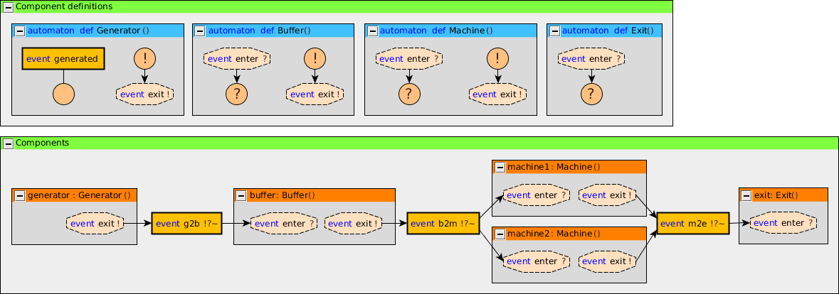
Using the Relations option (see the Options section above), certain kinds of relations included or excluded from the diagram. By default all kinds of relations are included. The following kinds of relations are available:
-
event relations (
event) -
data relations (
data)
In the option dialog, each of the features can be enabled and disabled individually, using a checkbox.
From the command line, using the -r or --relations option, the
names of the different kinds of relations, as indicates between parentheses
above, should be used, separated by commas. As an example, consider
-r event or --relations=event. Only the event relations are included,
while all the other relations are excluded.
The kinds that are specified using the option replace the default kinds.
However, it is also possible to specify additions and removals relative to the
default kinds, by prefixing names with a + or - respectively. For
instance, when using -r -event or --relations=-event the default kinds
are used, with the event relations excluded (due to -event). Replacements
(no prefix) may not be combined with additions/removals (+ or -
prefix).
Specifying a replacement kind type twice leads to a warning being printed to the console. Adding a kind that is already present or removing a kind that is not present, also leads to a warning being printed. Finally, generating a relations diagram without any relations also leads to a warning being printed.
Layout
The generated diagrams can be opened in the yEd Diagram Editor using . After opening the diagram, all nodes overlap, as the generated diagrams don’t contain any positions for them. yEd can automatically layout the diagram. Several layout algorithms are available in the Layout menu.
Good results for model diagrams can often be obtained by using the Orthogonal layout. Select to show the 'Orthogonal Layout' window. Click the Dock button to dock the window. Once docked, select Integrated for Edge Labeling and Free for Edge Label Model. Also enable the Length Reduction and Consider Node Labels options. Press the Apply changes button (the green rectangle) at the top of the docked window to apply the changes to the layout.
You may want to try different values for the 'Grid' option, to get more or less spacing between nodes. Once you change a value, just apply the new layout, as before. The automatic layout algorithms aren’t perfect, but they are usually a good starting point.
By default, edge labels have a light gray background. This makes them easier to read when placed on the edges. By changing the 'Edge Label Model' from 'Free' to 'Side Slider' , labels are not placed on the edges, but besides them. However, this often leads to some overlap, requiring manual layouting. If the 'Side Slider' variant is used, you may want to change the background of the edge labels to be transparent. This can be achieved by enabling the Transparent edge labels option (see the Options section above).
Good results for relations diagrams can often be obtained using the 'One-Click Layout' functionality of yEd. Select or use the corresponding toolbar button. This option is only available in yEd 3.14 or newer.
You can also close (collapse) and open (expand) groups and apply the layout again.
yEd has many more options. You can explore them using the included help text, by selecting .
Structure View
yEd has a Structure View window that can be enabled via . The Structure View can be used to see and navigate the structure of the CIF model. By switching from 'Text' to 'Description' (see upper right corner of the Structure View window), useful descriptions are shown for all elements. Furthermore, switching also ensures that the HTML code that is used for syntax highlighting is not shown in the Structure Viewer (if syntax highlighting is enabled, see the Options section above). The following image shows the difference:

Supervisory controller synthesis tools
Data-based supervisory controller synthesis
The data-based supervisory controller synthesis tool performs data-based supervisory controller synthesis, or simply data-based synthesis. It can be used to synthesize a supervisor for an untimed CIF specification, with data (e.g. discrete variables). For a CIF specification with plants and requirements, the tool computes a supervisor. The supervisor restricts the plants in such a way that the resulting controlled system satisfies the following properties:
-
The controlled system is safe. That is, all reachable states in the controlled system satisfy the requirements.
-
The controlled system is controllable. That is, for all reachable states in the controlled system, the uncontrollable events that are enabled in the same state in the uncontrolled system are still possible in the controlled system. In other words, uncontrollable events are not restricted.
-
The controlled system is non-blocking. That is, it is possible to reach a marked state from all reachable states in the controlled system.
-
The controlled system is maximally permissive (or simply maximal). That is, the controlled system permits all safe, controllable, and non-blocking behaviors.
Note that deadlock is not prevented for marked states.
The synthesis algorithm is based on the following paper: Lucien Ouedraogo, Ratnesh Kumar, Robi Malik, and Knut Åkesson: Nonblocking and Safe Control of Discrete-Event Systems Modeled as Extended Finite Automata, IEEE Transactions on Automation Science and Engineering, Volume 8, Issue 3, Pages 560-569, July 2011.
Starting the transformation
The transformation can be started in the following ways:
-
In Eclipse, right click a
.ciffile in the 'Project Explorer' tab or 'Package Explorer' tab and choose . -
In Eclipse, right click an open text editor for a
.ciffile and choose . -
Use the
cifdatasynthtool in a ToolDef script. See the scripting documentation and tools overview page for details. -
Use the
cifdatasynthcommand line tool.
Options
Besides the general application options, this application several other options.
The following options are part of the Synthesis category:
-
Input file path: The absolute or relative local file system path to the input CIF specification.
-
Output file path: The absolute or relative local file system path to the output CIF file. If not specified, defaults to the input file path, where the
.ciffile extension is removed (if present), and a.ctrlsys.ciffile extension is added. -
Supervisor name: The name of the resulting supervisor automaton. If not specified, it defaults to
sup. For more information, see the section on the resulting supervisor below. -
Supervisor namespace: The namespace of the resulting supervisor. If not specified, it defaults to the empty namespace. For more information, see the section on namespaces below.
-
Forward reachability: Whether to perform forward reachability during synthesis, or omit it. Is disabled by default. For more information, see the section on forward reachability below.
-
Statistics: The kinds of statistics to print. By default, no statistics are printed. For more information, see the section on statistics below.
Internally during synthesis, predicates are represented using Binary Decision Diagrams (BDDs). There are various options that can influence the use of BDDs. The following options are part of the BDD sub-category of the Synthesis category:
-
BDD output mode: This option can be used to control how the BDDs are converted to CIF for the output of synthesis. For more information, see the BDD representation in CIF section below.
-
BDD output name prefix: The prefix to use for BDD related names in the output. Only has an effect if the BDD output mode option is set to represent the internal BDD nodes directly in CIF. The default prefix is
bdd. For more information, see the BDD representation in CIF section below. -
BDD variable order: CIF variables and automata are represented using one or more boolean variables. The initial order of the boolean variables is determined by this option. For more information, see the BDD variable order section below.
-
BDD FORCE variable ordering algorithm: CIF variables and automata are represented using one or more boolean variables. The initial order of the boolean variables can be improved by enabling this option. For more information, see the BDD variable order section below.
-
BDD sliding window variable ordering algorithm: CIF variables and automata are represented using one or more boolean variables. The initial order of the boolean variables can be improved by enabling this option. For more information, see the BDD variable order section below.
-
BDD sliding window size: The maximum length of the window to use for the BDD sliding window variable ordering algorithm. This option only has effect if the BDD sliding window variable ordering algorithm option is enabled. The size must be an integer number in the range [1 .. 12]. The default size is 4. For more information, see the BDD variable order section below.
-
BDD predicate simplify: Several BDD predicates may be simplified under the assumption of other predicates, resulting in smaller/simpler output. This may decrease the size of the resulting controller, and may give more insight. For more information, see the Simplification section below.
-
BDD library initial node table size: The BDD library that is used maintains an internal node table. This option can be used to set the initial size of that node table. The size will automatically be increased during synthesis, if necessary. Increasing the initial size can increase performance for large systems, as it will not be necessary to repeatedly increase the size of the node table. However, a larger node table requires more memory, and can lead to the node table no longer fitting within CPU caches, degrading performance. The default is
100000nodes. The initial node table size must be in the range [1 .. 231 - 1]. For more information, see the Statistics section. -
BDD library operation cache size: The BDD library that is used maintains an internal operation cache. This option can be used to set the fixed size of that cache. The operation cache size must be in the range [2 .. 231 - 1]. By default, this option is disabled (value
offon the command line), and the BDD library operation cache ratio option is used instead. For more information, see the BDD operation caches section below. -
BDD library operation cache ratio: The BDD library that is used maintains an internal operation cache. This option can be used to set the ratio of the size of the operation cache of the BDD library to the size of the node table of the BDD library. For instance, a ratio of
0.1means that the size of the operation cache is 10% of the size of the node table. The operation cache ratio must be in the range [0.01 .. 1000]. The default ratio is 1.0. This option has no effect if the BDD library operation cache size option is enabled. For more information, see the BDD operation caches section below. -
BDD debug max nodes: Internally, predicates are represented using Binary Decision Diagrams (BDDs). This option control the maximum number of BDD nodes for which to convert a BDD to a readable CNF/DNF representation for the debug output. The default is
10nodes. The maximum must be in the range [1 .. 231 - 1]. The option can be set to have an infinite maximum (no maximum), using option valueinf. For more information, see the Debug output section below. -
BDD debug max paths: Internally, predicates are represented using Binary Decision Diagrams (BDDs). This option control the maximum number of BDD true paths for which to convert a BDD to a readable CNF/DNF representation for the debug output. The default is
10paths. The maximum must be in the range [0 .. 1.7e308]. The option can be set to have an infinite maximum (no maximum), using option valueinf. For more information, see the Debug output section below.
Supported specifications
The data-based supervisory controller synthesis tool supports a subset of CIF specifications. The following restrictions apply:
-
Only
plantandrequirementautomata are supported. Automata with asupervisorkind, as well as kindless/regular automata (without a supervisory kind) are not supported. -
Specifications without plant automata are not supported.
-
Events not declared as controllable or uncontrollable are not supported. This includes the
tauevent, both explicitly used on edges, as well as implicitly for edges without explicitly mentioned events. -
The use of channels (events with data types) in requirements is not supported. That is, requirements that send or receive (with or without data) are not supported.
-
Regular invariants, plant invariants, and supervisor invariants are not supported. Only requirement invariants are supported. To allow plant state/event exclusion invariants to be used in the input, manually eliminate them first using the Eliminate state/event exclusion invariants CIF to CIF transformation.
-
Continuous variables are not supported.
-
Only discrete/input variables with a boolean type, ranged integer type (e.g.
int[0..5]), or enumeration type are supported. For integer types, ranges that include negative integer values are not supported. For algebraic variables and algebraic parameters of components, all types are supported. -
Discrete variables must have supported initial values. If explicit initial values are given, they must be supported predicates (for boolean variables) or supported expressions as described below (for all other variables).
-
Automata with non-determinism for controllable events are not supported. That is, automata that have locations with multiple outgoing edges for the same controllable event, with overlapping guards (e.g.
x > 1andx < 4), are not supported. Note that this check is performed on the linearized guards, and may therefore lead to false positives, as the check is an over-approximation and guard overlap may be detected for unreachable states. -
Conditional updates (
ifupdates), multi-assignments, and partial variable assignments are not supported.
Only limited forms of predicates (for markers, invariants, initialization, guards, etc) are supported. The supported predicates are:
-
Boolean literals (
true,false). -
Discrete/input/algebraic boolean variables (
x, forxa discrete, input, or algebraic variable with a boolean type). -
Locations (
aut.loc, forautand automaton andloca location of that automaton). -
The unary inverse operator (
not) on a supported predicate. -
The binary logical conjunction (
and) on two supported predicates. -
The binary logical disjunction (
or) on two supported predicates. -
The binary logical implication (
=>) on two supported predicates. -
The binary logical bi-conditional (
<=>) on two supported predicates. -
The binary equality comparison (
=) on two supported predicates, or on two supported integer or enumeration expressions. -
The binary inequality comparison (
!=) on two supported predicates, or on two supported integer or enumeration expressions. -
The binary less than comparison (
<) on two supported integer expressions. -
The binary less than or equal comparison (
<=) on two supported integer expressions. -
The binary greater than comparison (
>) on two supported integer expressions. -
The binary greater than or equal comparison (
>=) on two supported integer expressions. -
Conditional expressions (
ifexpressions) with supported guard and resulting value predicates.
Only limited forms of integer and enumeration expressions (for binary comparisons, initial values of variables, right hand sides of assignments, etc) are supported. The supported expressions are:
-
A non-negative integer literal/value.
-
An enumeration literal/value.
-
Discrete/input/algebraic integer/enumeration variables (
x, forxa discrete, input, or algebraic variable with an integer or enumeration type). -
+iforia supported integer expression. -
i + jforiandjsupported integer expressions. -
i div jandi mod jforia supported integer expressions, andja positive integer value, or a computation that results in a positive integer value, as long as the computation is not too complex to be performed statically. That is,jmust essentially be constant. -
Conditional expressions (
ifexpressions) with supported guard predicates and supported resulting values. -
Any other valid CIF expression (computation) that that results in a non-negative integer value or an enumeration value, as long as the computation is not too complex to be performed statically. That is, the computation must essentially represent a fixed/constant value.
Here are some examples of computations that can be statically evaluated:
-
true and false(result isfalse) -
c or false, for a constantcwith valuefalse(result isfalse) -
1 + 1(result is2) -
2 * 5(result is10) -
floor(3.14)(result is3) -
c + 1, for a constantcwith value2(result is3)
Here are some examples of computations that can not be statically evaluated:
-
v + 1, forva discrete variable. The computation results in different values for different values ofv. -
v = trueforva discrete variable. The computation results in different values for different values ofv. -
v = eforva discrete variable andean enumeration literal/value. The computation results in different values for different values ofv.
Only limited forms of assignments are supported. The supported assignments are:
-
xb := p -
xi := ie -
xi := ie - ie -
xe := ee
For the following constraints:
-
xbis a boolean variable. -
xiis a supported integer variable, as described above. -
xeis an enumeration variable. -
pis a supported predicate, as described above. -
ieis a supported integer expression, as described above. -
eeis a supported enumeration expression, as described above.
Additionally, the tool warns about state/event exclusion invariants for events that are not in the alphabet of any automaton. Such invariants have no effect, as they try to (further) restrict events that are never enabled to begin with.
Preprocessing
The following CIF to CIF transformations are applied as preprocessing (in the given order), to increase the subset of CIF specifications that can be synthesized:
Additionally, the CIF specification is converted to an internal representation on which the synthesis is performed. This conversion also applies linearization (product variant) to the edges. Predicates are represented internally using Binary Decision Diagrams (BDDs).
Supported requirements
Three types of requirements are supported: state invariants, state/event exclusion invariants, and requirement automata.
State invariants are global conditions over the values of variables (and locations of automata) that must always hold. Such requirements are sometimes also called mutual state exclusions. Here are some examples:
requirement invariant x != 0 and not p.b;
requirement invariant x > 5;
requirement invariant not(x = 1 and y = 1) or q.x = a;

requirement (x = 1 and y = 1) or (x = 2 and y = 2);
requirement (3 <= x and x < = 5) or (2 <= y and y <= 7);
requirement x = 1 => y > 2;
State/event exclusion invariants or simply state/event exclusions are additional conditions under which transitions may take place for certain events. Here are some examples:
requirement invariant buffer.c_add    needs buffer.count < 5;
requirement invariant buffer.c_remove needs buffer.count > 0;
requirement invariant button.on = 1 disables lamp.c_turn_on;

requirement {lamp.c_turn_on, motor.c_turn_on} needs button.Off;
requirement p.x = 3 and p.y > 7 disables p.u_something;
Requirement automata are simply automata marked as requirement. They
usually introduce additional state by using multiple locations or a variable.
The additional state is used to be able to express the requirement. One common
example is a counter. For instance, consider the following requirement, which
prevents more than three products being added to a buffer:
requirement automaton counter:
  disc int[0..5] count = 0;

  requirement invariant count <= 3;

  location:
    initial;
    marked;

    edge buffer.c_add do count := count + 1;
end
Another common example is a requirement that introduces ordering. For instance,
consider the following requirement, which states that motor1 must always be
turned on before motor2 is turned on, and they must always be turned off in
the opposite order:
requirement automaton order:
  location on1:
    initial;
    marked;
    edge motor1.c_on goto on2;

  location on2:
    edge motor2.c_on goto off2;

  location off2:
    edge motor2.c_off goto off1;

  location off1:
    edge motor1.c_off goto on1;
end
Besides the explicit requirements, synthesis also prevents runtime errors. This
includes enforcing that integer variables stay within their range of allowed
values. This is essentially an implicit requirement. For instance, for a CIF
specification with a variable x of type int[0..5] and a variable y
of type int[1..3], requirement invariant
0 <= x and x <= 5 and 1 <= y and y <= 3 is
implicitly added and enforced by the synthesis algorithm. In the resulting
controlled system, no runtime errors due to variables being assigned values
outside their domain (integer value range) occur.
Resulting supervisor
If the supervisor has to restrict so much of the behavior of the uncontrolled system that no initial state remains, the controlled system becomes empty. The synthesis algorithm then ends with an empty supervisor error, and no output CIF file is created.
If an initial state remains after synthesis, an output CIF file is created. The
contents is the controlled system. The controlled system is obtained by taking
the input specification, and modifying it. The requirement automata are changed
to supervisor automata. Some or all of the requirement invariants may be
removed, depending on the
simplifications that are applied. An
additional external supervisor automaton is added. Also, depending on the
simplifications that are applied, the requirement automata may serve as
monitors or observers for the external
supervisor, or may actually impose the requirement restrictions. An external
supervisor is a supervisor automaton that adds restrictions to the
uncontrolled system (the plants), and potentially the requirement automata,
depending on the simplifications that are applied. The supervisor uses the
same events as the plants, and refers to plant and requirement locations and
variables in its conditions.
By default, the resulting external supervisor automaton is put in the empty namespace, at the top level of the resulting specification. That is, the supervisor automaton is not put in any groups. See the Namespace section for more information.
By default, the added supervisor automaton is named sup. Using the
Supervisor name option (see options section
above), it is possible to specify a different name. Custom supervisor automaton
names must be valid CIF identifiers, i.e. they may consist of letters, digits,
and underscores (_), but may not start with a digit. If the resulting
supervisor automaton has a name that conflicts with an existing declaration, it
is automatically renamed to have a non-conflicting name. In such cases, a
warning is printed to the console to inform the user.
The resulting supervisor has exactly one self loop edge for each of the controllable events in the alphabet of the controlled system (which is equal to the alphabet of the uncontrolled system). These self loops represent the possible conditions under which the supervisor allows the events to occur in the controlled system. The exact predicates may vary, depending on the simplifications that are applied.
The resulting supervisor may have an initialization predicate that restricts the states in which the system may be initialized (may start), on top of the initialization constraints already present in the uncontrolled system. For more information on this initialization predicate, see the section on initialization below.
Namespace
As indicated above, by default the resulting supervisor automaton is put in the empty namespace, at the top level of the resulting specification. That is, the supervisor automaton is not put in any groups.
It is possible to add a namespace to the entire resulting specification. That is, to put groups around the original plants and requirements, the added supervisor automaton, etc. A namespace can be added using the Supervisor namespace option (see options section above). By default, no additional namespace is added.
By adding a namespace around the entire resulting specification, the synthesis result can be easily merged with for instance a simulation model. The added namespace ensures that there are no naming conflicts between the plants of the simulation model and the similarly original plants. The events are not put in the new namespace, but are instead kept in their original place, wrapped in groups as necessary to keep their original identities (absolute names). This ensures that it remains possible to connect (merge) the events of the synthesis output with the events of the simulation model.
The namespace specified using the option, must consist of one or more valid CIF
identifiers, separated by dots (.). Valid CIF identifiers consist of one or
more letters, digits, and underscores (_), but may not start with a digit.
As an example, consider namespace a.b. A group b is wrapped around the
entire synthesis result, and a group a is wrapped around group b. Group
a is then the new synthesis result.
If a part of the namespace has the same name as an event that remains in its original place, this leads to a conflict, and synthesis fails. If the namespace does not conflict, but is non-empty (it contains an event or it contains a group that contains an event), synthesis also fails.
BDD representation in CIF
Internally, predicates are represented using Binary Decision Diagrams (BDDs). The supervisor that is the output of synthesis, contains several predicates as well. For instance, it has self loops with guard predicates, and it may have an initialization predicate. The predicates represented as BDDs need to be represented as CIF predicates. There are multiple approaches to do this, and the BDD output mode option (see options section above), can be used to configure the approach to use.
The first approach, which is also the default approach (named normal), is
to use either
Conjunctive Normal Form
(CNF) or
Disjunctive Normal Form
(DNF) predicates. This
approach has as benefit that for relatively small predicates (usually for small
systems), the CIF predicates are often intuitive, and can easily understood.
The downside is that for larger systems, the CIF predicates often grow
exponentially in size.
The second approached (named nodes), is to represent the internal BDD nodes
directly in CIF. The BDD is then more or less coded directly in CIF, using
some constants and algebraic variables, and is evaluated using a BDD evaluation
function. The benefit is that for larger systems, this representation remains
relatively small, and at the very least doesn’t blow up nearly as much as the
CNF and DNF representations. The downside to this approach, is that it leads to
a supervisor that can not be easily understood by inspecting it. For this
approach, several objects are created in the top level scope of the CIF
specification. The names of these declarations all share a common prefix. The
default prefix is bdd, but it can be changed using the
BDD output name prefix option (see
options section above). No existing
declarations, whose names start with that prefix, should be present in the top
level scope of the specification.
Initialization
The synthesis algorithm ensures that in the controlled system, the requirement state invariants hold in all reachable states. It also ensures that in the controlled system, for all transitions from reachable states, the events only occur if the requirement automata and state/event exclusion invariants allow them.
The synthesis algorithm does not restrict any uncontrollable events. Instead, such restrictions are propagated backwards to the source state of the edge with the uncontrollable event, and from there to the transitions that lead to the source state, etc. They are propagated backwards until an edge with a controllable event is encountered (for which the guard can be restricted) or the initial state is reached (and the initialization predicate can be restricted).
If a variable in the uncontrolled system has a single initial value, and the initialization predicate is restricted to not allow this initial value, initialization will be impossible, causing an empty supervisor error. For discrete variables with multiple potential initial values, the synthesis algorithm may restrict initialization to disallow certain initial values, while still leaving possibilities for initialization. For discrete variables declared to initially have an arbitrary initial value, as well as for input variables, the synthesis algorithm essentially determines under which conditions the system can be started, and still exhibits only safe, non-blocking behavior.
If the controlled system requires more strict initialization than the uncontrolled system, an additional initialization predicate is added to the resulting supervisor. The exact predicate may differ, depending on the simplifications that are applied.
Forward reachability
Synthesis essentially works by calculations that involve predicates that partition the entire state space into states that satisfy a property or don’t satisfy a property. For instance, a marker predicate may indicate which states of the state space are marked. All other states are thus not marked.
Calculations during synthesis often involve reachability. For instance, from which states is it possible to reach a marker state? To compute the states that can reach a marker state, the marker predicate of the input specification is used. The marker predicate indicates the states that are themselves marked. Then, the states are calculated that can reach one of those marked states, via a single transition. They are put together, to form the states that are marked or can be marked after one transition. By taking another such step, we can add the states that can reach a marked state via two transitions. We then have all states that can reach a marked state via zero, one, or two transitions. We can repeat this until no new states are found, which is called reaching a fixed point.
This form of reachability is called backward reachability, as it starts with some target (e.g. marked states), and goes backwards to find all states from which the target can be reached. Backward reachability can lead to states that could never be reached from an initial state, even in the uncontrolled system. This leads to two separate issues.
The first issue is about unintuitive resulting supervisor guards. The resulting supervisor forbids certain transitions, by restricting controllable events. It among others forbids transitions that end up in states from which no marked state can be reached. However, if those forbidden states can never be reached from an initial state, there is no reason to restrict the controllable events in such cases. The guards of the resulting supervisor then appear to restrict the controllable events, while in fact the guard doesn’t impose a restriction for the controlled system. The supervisor simply doesn’t have the necessary information to know this.
The second issue is about performance. Expanding unreachable states during backward reachability takes time and costs memory, while it has no useful effect on the resulting controlled system.
The use of forward reachability can be a solution to both problems. Forward reachability starts with the initial states, and adds states reachable via one transitions, then via two transitions, then via three transitions, etc. This is repeated until all reachable states are found.
By combining both forward and backward reachability, the supervisor knows about states that exist in the uncontrolled system (due to forward reachability) and about states that it should forbid (due to backward reachability). This leads to the supervisor only restricting transitions that are strictly necessary. However, both when using forward reachability and when not using it, the synthesized supervisor is safe, non-blocking, and maximally permissive. It is only the guards that are more complex than they might need to be, if forward reachability is not used. More complex guards are often less readable, and potentially more expensive to implement in an actual controller.
By combining both forward and backward reachability, parts of the state space that are not relevant may not have to be expanded (as much), which may improve performance. However, computing the forward reachability may also take time and cost memory, thus reducing performance.
It depends on the specification being synthesized whether enabling forward reachability increases or decreases performance. It also depends on the specification whether there is any benefit to using forward reachability for the guards of the supervisor. Forward reachability is disabled by default. It can be enabled using the Forward reachability option (see options section above).
Simplification
The synthesis algorithm computes various predicates, such as the conditions under which the controllable events may take place in the controlled system, and the initialization predicate of the controlled system. These predicates are included in the supervisor that results from synthesis.
However, if the controlled system imposes the exact same restrictions as the
uncontrolled system, there is no need to list the full conditions in the
supervisor, as the plants already define that behavior. The supervisor imposes
no additional restrictions with respect to the plants, and it suffices to use
true as condition for the supervisor to make that explicit.
There are several predicates in the synthesis result that can be simplified under the assumption of conditions that are already present in the input specification. In some cases this leads to smaller/simpler supervisor representations. In other cases it gives insight, indicating that the supervisor does not impose any additional restrictions. The following simplifications are available:
| Option value | Default | Predicate | May be simplified assuming |
|---|---|---|---|
|
yes |
Supervisor guards of controllable events |
Plant guards, for the matching events |
|
yes |
Supervisor guards of controllable events |
State/event exclusion requirement invariants derived from the requirement automata, for the matching events |
|
yes |
Supervisor guards of controllable events |
State/event exclusion requirement invariants from the input specification, for the matching events |
|
yes |
Supervisor guards of controllable events |
State requirement invariants from the input specification (includes the range requirement invariants added by the synthesis algorithm) |
|
yes |
Supervisor guards of controllable events |
Controlled behavior as computed by synthesis |
|
yes |
Initialization predicate of the controlled system |
Initialization predicate of the uncontrolled system |
Which simplifications should be performed, can be specified using the BDD predicate simplify option (see options section above).
The table above lists in the first column, the option values to use for each of
the simplifications, on the command line. The names given in the first column
should be combined using commas, and used as option value. The simplifications
that are specified using the option replace the default simplifications (see
the second column of the table). However, it is also possible to specify
additions and removals relative to the default simplifications, by prefixing
simplifications (from the first column) with a + or - respectively.
Replacements (no prefix) may not be combined with additions/removals (+ or
- prefix). Specifying a simplification twice leads to a warning being
printed to the console. Adding a simplification that is already present or
removing a simplification that is not present, also leads to a warning being
printed.
In the option dialog, each of the simplifications can be enabled or disabled using a checkbox.
The second column indicates for each simplification whether it is enabled by default. By default, all simplifications are enabled. The third column indicates the predicate in the synthesis result that can be simplified. The fourth column indicates under the assumption of which predicate the simplification is applied.
The simplification algorithm is not perfect, and may not simplify the predicates as much as could potentially be possible.
When simplifying with respect to state requirement invariants, the supervisor no longer enforces those requirements, as they are assumed to already hold. As such, the simplification prevents such invariants from being removed from the resulting CIF specification. This applies to some of the other simplifications as well. For instance, the simplification over state/event exclusion requirement invariants leads to them being part of the output as well. This may affect whether other tools can handle the resulting supervisor model as input, depending on what kind of features they support. In particular, for code generation, simplification of the guards with respect to the state requirement invariants and state/event exclusion requirement invariants may need to be disabled.
Debug output
By default, the synthesis algorithm shows no progress information, and does not explain how the resulting supervisor is obtained. By enabling debug output, detailed information is printed to the console. Debug output can be enabled by setting the Output mode option (General category) to Debug.
The debug output also contains information about the number of states in the
resulting controlled system (the uncontrolled system restricted by the
synthesized supervisor). If the resulting supervisor (and thus the controlled
system) is empty, or if
forward reachability is enabled, the
number of states that is printed is an exact number (e.g. exactly 0 states,
exactly 1 state, exactly 1,234 states). In other situations, the
controlled behavior predicate that is used to determine the number potentially
gives an over-approximation, and an upper bound on the number of states is
printed (e.g. at most 1,234 states).
Enabling debug output may significantly slow down the synthesis algorithm, especially for larger models. The performance degradation stems mostly from the printing of predicates. Predicates are internally represented using Binary Decision Diagrams (BDDs). To print them, they are converted to CNF or DNF predicates, similar to one of the approaches to convert BDDs to CIF predicates for synthesis output.
To limit the performance degradation, options are available to limit the
conversion of BDDs to CNF/DNF predicates. The BDD debug max nodes controls
the maximum number of BDD nodes for which to convert a BDD to a readable
CNF/DNF representation for the debug output. The default is 10 nodes. The
maximum must be in the range [1 .. 231 - 1].
The option can be set to
have an infinite maximum (no maximum), using option value inf. The BDD
debug max paths option controls the maximum number of BDD true paths for which
to convert a BDD to a readable CNF/DNF representation for the debug output. The
default is 10 paths. The maximum must be in the range [1 .. 1.7e308]. The
option can be set to have an infinite maximum (no maximum), using option value
inf. If a BDD has more than the specified maximum number of nodes, or more
than the specified number of true paths, it is not converted to a CNF/DNF
predicate. Instead, it is converted to a textual representation that indicates
the number of nodes and true paths, e.g. <bdd 1,234n 5,678p> for a BDD with
1,234 nodes and 5,678 true paths.
By limiting the conversion of BDDs to CNF/DNF predicates, debug output can still be used for large models to see progress information, while not degrading the performance too much.
Statistics
The data-based synthesis tool supports printing various kinds of statistics to the console. By default, no statistics are printed. Statistics can be enabled using the the Statistics option (see options section above). The following statistics are available:
-
Timing [
timing]Print statistics for timing of various parts of the tool. Is printed to the console, after execution, just termination of the tool. Timing is only printed for parts of the tool that were actually executed. Timing is printed as a tree. The root of the tree represents the total time of the synthesis tool. For some parts of the tool, timing is also measured for sub-parts. Timing is printed in milliseconds, to make it easier to compare timing for various parts.
When measuring performance, always perform multiple measurements, and take the average. Also, use a warm-up phase, to avoid skewed results.
-
BDD garbage collection [
bdd-gc]The BDD library that is used maintains an internal node table. Whenever new nodes no longer fit in the node table, a garbage collection is started by the BDD library, to clean out all nodes that are no longer needed. BDD garbage collection statistics are printed before and after garbage collection. The printed information includes the size of the node table, the number of free nodes, timing information, etc. See also the BDD library initial node table size option (see options` section above).
-
BDD node table resize [
bdd-resize]The BDD library that is used maintains an internal node table. Whenever new nodes no longer fit in the node table, a garbage collection is started by the BDD library, to clean out all nodes that are no longer needed. If only very limited space could be reclaimed by garbage collection, the size of the node table is increased. BDD node table resize statistics are printed when the node table is resized. The printed information includes the old and the new sizes of the node table. See also the BDD library initial node table size option (see options` section above).
In the option dialog, each of the different kinds of statistics can be enabled and disabled individually, using a checkbox.
From the command line, using the --stats option, the names of the different
kinds of statistics, as indicated above between square brackets, should be
used, separated by commas. For instance, use --stats=bdd-gc,bdd-resize to
enable both BDD garbage collection statistics and BDD node table resize
statistics, but keep all other statistics disabled.
Specifying a statistics kind twice leads to a warning being printed to the console.
Early problem detection
The synthesis algorithm checks the uncontrolled system for common issues, for early detection of problems that will lead to an empty supervisor. If such a problem is detected, a warning is printed to the console. Among others, checks are included for no initial states/variables, no marked states, and no states due to the invariants.
BDD variable order
Internally, predicates are represented using
Binary Decision Diagrams
(BDDs). CIF
variables and automata are represented using one or more boolean variables
(also called BDD variables or bits). For instance, a boolean CIF variable is
represented using a single boolean/BDD variable, and a CIF variable of type
int[0..8] is represented using four boolean/BDD variables (9 possible
values, log2(9) ≈ 3.17). For each automaton with two or
more locations, a location pointer variable is created, that represents the
current or active location of that automaton. For instance, an automaton with
three locations is represented using two boolean/BDD variables. Two boolean/BDD
variables can represent 22 = 4 values, so one value is not
used.
The CIF variables and location pointer variables for the automata
(together called synthesis variables) can be ordered. This ordering can
significantly influence the performance of synthesis. Synthesis variables that
have a higher influence on the result of predicates (simply put, occur more
frequently in predicates) should generally be put earlier in the ordering.
Furthermore, in general, strongly related synthesis variables (e.g. by
comparison, integer computation, or assignment) should be kept closely together
in the order. For two synthesis variables x and y, examples of
predicates that introduce relations are x = y (by comparison) and
5 < x + y (by integer computation), and examples of assignments that
introduce relations are x := y and x := y + 1 (both by assignment).
For the initial variable ordering, it is possible to order the BDD variables per synthesis variable, or to interleave the BDD/boolean variables of some synthesis variables. This can significantly influences the performance of synthesis. Generally, strongly related synthesis variables should be interleaved.
For more information on ordering and its influence on performance, see Chapter 3 of [minato].
For each CIF variable and location pointer, two synthesis variables are created, one storing the old/current value (before a transition), and one storing the new value (after a transition). For a single CIF variable or location pointer, the old and new synthesis variables are always kept together, and interleaved. The old synthesis variable is also always before the new synthesis variable.
The initial order of the boolean/BDD variables is determined by the BDD variable order option (see options section above). Several default orders exist, and it is also possible to define a custom order. By default, the sorted order is used. The following default orders exist:
-
model ordering without interleaving (option value
model)The initial order of the synthesis variables is as they occur in the model. A location pointer, for an automaton with two or more locations, is put before the variables declared in that automaton.
No synthesis variables are interleaved, except for each old variable with its corresponding new variable.
-
reverse model ordering without interleaving (option value
reverse-model)The initial order of the synthesis variables is as they occur in the model, but reversed. A location pointer, for an automaton with two or more locations, is put after the variables declared in that automaton, in this reverse order.
No synthesis variables are interleaved, except for each old variable with its corresponding new variable. The old variables are still before the new variables; this is not reversed.
-
sorted ordering without interleaving (option value
sorted)The initial order of the synthesis variables is based on the names of the variables and automata. They are sorted alphabetically in ascending order, based on their absolute names.
No synthesis variables are interleaved, except for each old variable with its corresponding new variable.
-
reverse sorted ordering without interleaving (option value
reverse-sorted)The initial order of the synthesis variables is based on the names of the variables and automata. They are sorted alphabetically in descending order, based on their absolute names.
No synthesis variables are interleaved, except for each old variable with its corresponding new variable. The old variables are still before the new variables; this is not reversed.
-
random ordering without interleaving (option value
randomorrandom:SEED)The variables and automata are initially ordered randomly. If no seed is specified, a random seed is used, resulting in a random random order. If a seed is specified, a fixed random order is used. That is, using the same seed again, results in the same random order. The
SEEDmust be an integer number in the range [0 .. 264 - 1]. For instance, userandom:123as option value to get a random order that can be repeated on a subsequent synthesis for the same model.No synthesis variables are interleaved, except for each old variable with its corresponding new variable.
Furthermore, a custom initial order can be defined. Custom orders consist of
absolute names of variables and automata. That is, for an automaton
a, with a discrete variable x, the absolute name of the variable is
a.x. The * character can be used as wildcard in those names, and
indicates zero or more characters. In case of multiple matches, the matches are
sorted increasingly on their absolute names, and interleaved.
Multiple names can be separated with ; characters. The synthesis variables
matching the name pattern before the ; are ordered before the synthesis
variables matching the name pattern after the ;. The ; separator does
not introduce interleaving. The , separator can be used instead of the
; separator to introduce order but also introduce interleaving.
Each name pattern in the order must match at least one variable or automaton. A variable or automaton may not be included more than once in the order. Every variable and automaton (with two or more locations) needs to be included in the order. It is not possible to specify new variables, as they are always directly after their corresponding old variables, and they are always interleaved.
For instance, consider two automata: a and b, each with three
variables of type int[0..3]: x1, x2, and x3. The automata have
three locations each, so location pointers are created for them. We thus have
six discrete variables: a.x1, a.x2, a.x3, b.x1, b.x2, and
b.x3, and two location pointer variables: a and b. Consider the
following custom order: b*;a.x3,a.x1;a.x2,a. Pattern b* matches
location pointer variable b as well as the three discrete variables of
automaton b (b.x1, b.x2, and b.x3). They are ordered in
increasing alphabetic order, and are interleaved. Variables a.x3 and
a.x1 are also interleaved, with a.x3 before a.x1. Finally, variable
a.x2 is ordered before the location pointer for automaton a, and they
are interleaved as well. This results in the following initial boolean/BDD
variable ordering, with bits whose name ends with + representing bits of
new variables rather than current/old variables, and x#0 representing bit
zero of variable x:
b#0
b+#0
b.x1#0
b.x1+#0
b.x2#0
b.x2+#0
b.x3#0
b.x3+#0
b#1
b+#1
b.x1#1
b.x1+#1
b.x2#1
b.x2+#1
b.x3#1
b.x3+#1
a.x3#0
a.x3+#0
a.x1#0
a.x1+#0
a.x3#1
a.x3+#1
a.x1#1
a.x1+#1
a.x2#0
a.x2+#0
a#0
a+#0
a.x2#1
a.x2+#1
a#1
a+#1
The default orders are often not optimal performance-wise. Manually specifying a custom order often requires specialist knowledge and can take quite some time. Luckily, there are algorithms that can automatically compute a decent variable order.
The algorithms all take an initial variable ordering, and try to improve it using a fast heuristic. A better initial variable ordering may result in a better final variable ordering (a better local optimum), and may speed up the automatic variable ordering algorithm (reaching an optimum faster).
For the initial variable ordering, the CIF variables and location pointers may be arbitrarily interleaved. If an automatic variable ordering algorithm changes the initial order, no synthesis variables are interleaved, except for each old variable with its corresponding new variable.
The automatic variable ordering algorithms are not applied if the CIF model has less than two synthesis variables. They are also not applied if the model has no guards, updates, or other predicates to use as input for the algorithms, i.e. there are no hyperedges to which to apply the algorithms.
The following algorithms are available:
-
FORCE
The [force] algorithm is enabled by default, but can be disabled using the BDD FORCE variable ordering algorithm option (see options section above).
At most 10 * ceil(loge(n)) iterations of the FORCE algorithm are performed, with
nthe number of current/old BDD/boolean variables. -
Sliding window
The sliding window algorithm is enabled by default, but can be disabled using the BDD sliding window variable ordering algorithm option (see options section above).
The default maximum length of the window that is used is 4. The actual window may be smaller, if less than 4 variables and/or location pointers are present in the model. The maximum length of the window can be configured using the BDD sliding window size option (see options section above). The option to set the maximum length only has effect if the sliding window variable ordering algorithm is enabled. The size must be an integer number in the range [1 .. 12].
If enabled, the algorithms are applied in the order they are listed above.
BDD operation caches
One of the main properties of BDDs is that they employ full sharing. That is, if a part of a binary tree needs to be represented more than once, it is stored only once, and reused. This leads to BDDs being represented using directed acyclic graphs, rather than binary trees.
The BDD library uses an operation cache to speed up synthesis. Whenever a certain operation is performed on one or more nodes of a BDD graph, the result is cached. If that same operation is performed again on the same nodes, the cached result is reused, if available. This way, repeated calculations can be prevented for shared sub-graphs.
The operation cache is essential for the performance of the synthesis algorithm. With infinite caches, the operations are generally linear in the number of nodes used to represent the BDDs on which they are applied. Without caching, the computation time grows exponentially.
Obviously, in practice we can’t have infinite caches, as a computer only has a finite amount of memory available. We thus need to work with finite caches. Whenever a new cached operation result doesn’t fit in the cache, an older result is overwritten, and will need to be recomputed if it is needed again.
Increasing the cache size can significantly increase performance for large systems, as a cache that is too small is ineffective, and results in many operations needing to be repeated, that could have otherwise been obtained from the cache. However, a larger than needed cache may also significantly decrease performance, as a cache that is too large may no longer fit within CPU caches, leading to more expensive accesses to the main memory rather than e.g. L1/L2/L3 caches.
The operation cache size can be configured in two ways: as a fixed size that remains the same during the entire synthesis, or a variable cache size that grows in size as the node table grows in size. See the options section above for details.
Performance
The following options have an effect on the performance of data-based synthesis:
| Kind | Option | Section | Effect | Choose |
|---|---|---|---|---|
Output |
BDD output mode |
Representation of BDDs in the output model |
Use |
|
Output |
BDD predicate simplify |
Potentially smaller BDDs in the output |
Enable for smaller output, although simplification itself also takes time |
|
Order |
BDD variable order |
Better order for smaller BDD representations |
Choose the best order, depends on the model, (reversed) model/sorted usually good choices, custom order allows for best performance |
|
Order |
BDD FORCE variable ordering algorithm |
Better order for smaller BDD representations |
Enable for automatic ordering |
|
Order |
BDD sliding window variable ordering algorithm |
Better order for smaller BDD representations |
Enable for automatic ordering |
|
Order |
BDD sliding window size |
Better order for smaller BDD representations |
Larger windows might allow for more optimization, but take more time |
|
Library |
BDD library initial node table size |
More storage for less resizes |
Increase size for less resizes, at the cost of less memory locality |
|
Library |
BDD library operation cache size/ratio |
Increase cache for less computations |
Enable, larger costs more memory, larger leads to less memory locality, size/ratio depends on model |
|
Algorithm |
Forward reachability |
Explore only reachable state space |
Enable to reduce state space, although calculation itself may also be expensive, depends on model |
|
Debug |
Output mode |
Debug output on console |
Disable for better performance |
|
Debug |
BDD debug max nodes/paths |
Size of predicates in debug output |
The smaller, the less blowup, the better the performance |
|
Debug |
Statistics |
Statistics output on console |
Disable for better performance |
The first column categorizes the different options a bit, for different kind of options. The second column lists the different options. The third column indicates in which section on this page of the documentation you can find more information about that option. The fourth column indicates the effect of the option. The fifth column indicates what to choose for the option, for best performance, although a trade-off may be involved.
Obviously, the actual model that is used has a large impact as well. More variables often leads to longer synthesis times. However, the predicates that are used may also significantly impact performance.
Try to use state/event exclusion requirement invariants instead of requirement automata with a single location and self loops. Also, try to avoid an event-based modeling style, and use a data-based modeling style instead, if possible.
Input variables
Data-based synthesis supports input variables. The model itself doesn’t specify which value an input variable has at any given moment. Input variables can thus have any value (as long as it fits within the data type of the variable), and the value can change at any time. Input variables are ideal to model sensors.
To support this for data-based synthesis, the input variable is treated as a
discrete variable with an arbitrary initial value. To allow the input variable
to arbitrarily change, an uncontrollable event is added (with the same absolute
name as the input variable). Also, a single edge is added for that event. The
edge is always enabled (guard true, since the input variable can always
change value), and the update indicates that it can get any value that it
doesn’t currently have (x+ != x for x an input variable, with x
the value of the variable before the update, and x+ the value of the
variable after the update). Obviously, the value of the input variable is kept
within the range of values that is allowed by its data type.
Using synthesis with requirements that restrict the allowed values of an input variable will result in an empty supervisor, as a supervisor can’t prevent the environment from changing the value of the input variable (it would have to restrict the uncontrollable event that is internally added to model value changes of the input variable). A supervisor can however impose additional restrictions on the initial value of an input variable. The supervisor can then only guarantee safe, non-blocking behavior if the system is initialized in accordance with the additional initialization restrictions.
References
-
[minato] Shin-ichi Minato. Binary Decision Diagrams and Applications for VLSI CAD: The Springer International Series in Engineering and Computer Science, Volume 342, 1996, Springer US, ISBN 978-1-4613-1303-8 (E-book), ISBN 978-0-7923-9652-9 (hardcover), ISBN 978-1-4612-8558-8 (softcover)
-
[force] Fadi A. Aloul, Igor L. Markov, Karem A. Sakallah. FORCE: A Fast and Easy-To-Implement Variable-Ordering Heuristic: GLSVLSI '03 Proceedings of the 13th ACM Great Lakes symposium on VLSI pages 116-119, 2003, ACM New York, NY, USA, ISBN 1-58113-677-3
Event-based synthesis toolset
Synthesis, 'supervisor synthesis', or 'supervisory controller synthesis', is a generative technique, where one derives a (supervisor) automaton from a collection of plants and requirements. The resulting supervisor is maximally permissive under the conditions of being free of deadlocks, and always having the option of reaching a marked state.
While there is only one true synthesis tool (the tool that actually derives a supervisor automaton from a collection of plant and requirement automata), other tools exist to support the process. These tools together form the event-based synthesis toolset.
These tools use and modify the sequences of events that can be performed. This in contrast to state-based tools, which operate primarily on the state of the system. Event sequences directly hook into language theory, which places these tools firmly in the language theory mathematical framework.
Supported specifications
The application supports a subset of CIF specifications. The following restrictions apply:
-
Channels (events with data types), if used (present on an edge of at least one automaton), are not supported.
-
Any use of the
tauevent is not supported. Note that both explicit use (keywordtau) and implicit use (no events on an edge) are unsupported. -
Automata with multiple initial locations are not supported.
-
Edges with updates are not supported.
-
Urgent locations and edges are not supported.
-
Initialization predicates in components are not supported.
-
Invariants in components are not supported.
-
Marker predicates in components are not supported.
-
Initialization predicates in locations that are not trivially true or false are not supported.
-
State invariants in locations that are not trivially true are not supported.
-
Marker predicates in locations that are not trivially true or false are not supported.
-
State/event exclusion invariants are not supported.
-
Guards of edges that are not trivially true or false are not supported.
-
Multiple initialization predicates in a single location are not supported.
-
Multiple state invariant predicates in a single location are not supported.
-
Multiple marker predicates in a single location are not supported.
-
Multiple guards on a single edge are not supported.
To allow state/event exclusion invariants to be used in the input, manually eliminate them first using the Eliminate state/event exclusion invariants CIF to CIF transformation.
For meaningful results, it is recommended to have an initial location and at least one marked location, in each automaton.
Preprocessing
The following CIF to CIF transformations are applied as preprocessing (in the given order), to increase the subset of CIF specifications that can be transformed:
Automaton kinds
The event-based toolset recognizes the CIF automaton kinds plant,
requirement, and supervisor, and interprets them using the
corresponding concepts of the mathematical framework of supervisor synthesis.
Kindless/regular automata (without a supervisory kind) are treated as unknown.
Location names in reports and errors
Several tools output reports or give errors with locations that are interesting in some way.
Tools that take a single automaton as input report locations by their name in
the input specification, for example location "button.off" denotes the
off location in the button automaton. The location of automata that
have a single unnamed location use * as location name, for example
location "req.*" denotes the single unnamed location in the req
automaton.
Tools that take a number of automata together, like supervisor synthesis
report interesting states as state followed by the names of the locations,
for example state "button.on", "machine.idle". Such a state refers to a
location that represents the combined locations of the automata, in the
example, the combined locations button.off and machine.idle.
Tools that combine or merge locations, like projection, report such combined
locations as a partition, for example partition "machine.down",
"machine.off" represents a location that is a combination of the down
and the off locations in the machine automaton.
Available tools
-
Event-based synchronous product
Computes the product of a number of deterministic or non-deterministic automata, where common events are synchronized. Essentially computes the state space.
-
Event-based supervisor synthesis
Derivation of a maximal permissive supervisor from a collection of deterministic plant and requirement automata.
-
Event-based synthesis analysis
Analysis of the removed parts of a synthesized supervisor.
-
Event-based nonconflicting check
Verifies whether automata are conflicting, that is together could lead to non-coreachable states.
-
Event-based controllability check
Verifies whether the supervisor does not disable uncontrollable events of the plant.
-
Event-based language equivalence check
Verifies whether two automata produce the same events at each point.
-
Event-based NFA to DFA automaton conversion
Converts a non-deterministic automaton to a deterministic automaton while preserving the event behavior.
-
Minimize the number of locations of an automaton while preserving the event behavior.
-
Event-based automaton projection
Computes a projection of an automaton, resulting in a deterministic and language equivalent automaton over a subset of its alphabet.
-
Verifies whether an automaton can act as an observer of occurrences of observable events.
-
Event-based automaton abstraction
Abstracts an automaton to a set of observable events.
-
Verifies whether the automata are trim, that is, in each automaton, the locations must be both reachable and co-reachable.
-
Removes all locations that are not reachable or coreachable.
Event-based synchronous product
The event-based synchronous product takes one or more plant or requirement automata, and computes the synchronous product. Synchronous product means events on edges can only be taken if all automata with that event in their alphabet can take an edge with the same event at that time. This tool essentially computes the state space.
The tool takes a .cif file containing all automata to combine, and
produces a new .cif file with the product automaton. If the
kinds of the source automata are all the same,
the resulting product automaton is of that kinds as well. Otherwise, the
product automaton has unknown kind.
Starting the synchronous product tool
The tool can be started in the following ways:
-
In Eclipse, right click a
.ciffile in the 'Project Explorer' tab or 'Package Explorer' tab and choose . -
In Eclipse, right click an open text editor for a
.ciffile and choose . -
Use the
cifprodtool in a ToolDef script. See the scripting documentation and tools overview page for details. -
Use the
cifprodcommand line tool.
Options
Besides the general application options, this application has the following options:
-
Input file: The absolute or relative local file system path to the input CIF specification.
-
Output file: The absolute or relative local file system path to the output CIF specification. If not specified, defaults to the input file path, where the
.ciffile extension is removed (if present), and a_product.ciffile extension is added. Theproductpart of the default extension depends on the Result name option. -
Result name: The name to use for the product automaton. If not specified, defaults to
product. Also affects the Output file option.
Event-based supervisor synthesis
The supervisor synthesis procedure takes one or more deterministic plant automata, one or more deterministic requirement automata, and combines them to a maximal permissive supervisor.
The tool takes a .cif file containing plant and requirement
automata. Besides the general event-based restrictions listed at
Supported specifications, the current implementation
does not support:
-
Having no
plantautomata at all. -
Having no
requirementautomata at all. -
Having any other kind of automaton in the file. See Automaton kinds for a list of all automaton kinds.
-
Non-determinism in the input automata. The tool reports the violating automaton, location, and event, for ease of reference.
-
Events in the alphabet of the requirements that are not in the alphabet of the plants.
-
Events that are not controllable or uncontrollable, if used (present in the alphabet or on an edge of at least one automaton).
In addition, it warns about common mistakes:
-
Automata without a marked location.
-
Non-trim automata.
Finally, it can also perform checks about correct constructs that may not be the intention of its author. Each of these checks has to be enabled with an option:
-
Automata with a marked deadlock location. In a system with infinite behavior, you should probably never enter a deadlock location.
-
Automata with an empty alphabet. Such automata never participate in an event, and can be removed.
-
Controllable events that are used in exactly one automaton. Not always wrong, but creating a controllable event, and not using it for control may be a mistake.
-
Groups of automata that share events only within the group (and not with any automaton outside the group). Such a group is completely independent, and can be synthesized separately.
The synthesis tool produces a new .cif file with the supervisor
automaton (of kind supervisor) if the resulting automaton has at
least an initial location. Otherwise, synthesis fails with a Supervisor is
empty error, and no .cif file is written.
Starting the supervisor synthesis tool
The tool can be started in the following ways:
-
In Eclipse, right click a
.ciffile in the 'Project Explorer' tab or 'Package Explorer' tab and choose . -
In Eclipse, right click an open text editor for a
.ciffile and choose . -
Use the
cifsupsynthtool in a ToolDef script. See the scripting documentation and tools overview page for details. -
Use the
cifsupsynthcommand line tool.
Options
Besides the general application options, this application has the following options:
-
Input file: The absolute or relative local file system path to the input CIF specification.
-
Output file: The absolute or relative local file system path to the output CIF specification. If not specified, defaults to the input file path, where the
.ciffile extension is removed (if present), and a_sup.ciffile extension is added. Thesuppart of the default extension depends on the Result name option. -
Result name: The name to use for the supervisor automaton. If not specified, defaults to
sup. Also affects the Output file option. -
Enable Synthesis dump: If enabled, the synthesis algorithm writes a dump file containing the actions performed by the algorithm, for later analysis. The name of the file is decided by the Dump file option.
-
Synthesis dump file: The name of the dump file. Setting this option will enable dumping of the synthesis algorithm actions. The options contains the absolute or relative local file system path to the synthesis dump file. If not specified, defaults to the input file path, where the
.ciffile extension is removed (if present), and a.synth_dumpfile extension is added. -
Disjunct groups check: If enabled, the tool will report about groups of automata that share events in the group only.
-
Empty alphabet check: If enabled, the tool will report about automata without events in their alphabet.
-
Marked deadlock location check: If enabled, the tool will report about marked locations without outgoing edges.
-
Single use controllable check: If enabled, the tool will report about controllable events that are used in exactly one automaton.
Event-based synthesis analysis
While developing a controller with supervisory controller synthesis, the result is not always what you expect. To assist, the synthesis analysis tool has been developed. Its primary purpose is to explain why certain states or edges have been removed.
To use the tool, enable creation of the Synthesis Dump file during synthesis, using the Enable Synthesis dump option or the Synthesis dump file option of the Supervisor synthesis tool.
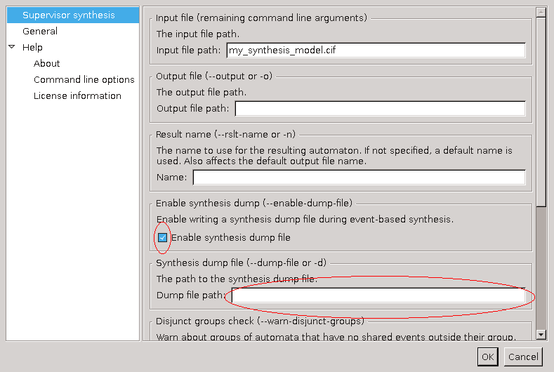
By double clicking the generated dump file, or by right-clicking the dump file and selecting Analyze Synthesis Result, the analysis tool is started. It loads the file (which can take a some time if the file is big), eventually giving the following display:

At the left, all automata with their initial location are shown. You can select a different supervisor state by changing these locations. At the top, in the middle, there are three buttons. The bottom button labeled Search state is used to search the information about a supervisor state selected at the left. The Jump to initial state button resets the automata locations to their initial state, useful when you want to start again. The middle button is disabled now, but allows you to go back to the previous state.
At the right, a number of options are available in case the displayed information is not sufficient. These are explained later.
Below the buttons and options is the report area, which just displays some statistics. When you press Search, the tool analyzes the selected state at the left. Depending on what happened with that state, different things may be shown. In this example, you get:

The report area changes to display the information about the selected state.
It starts with the internal number of this state (#0), and its properties.
The initial means this state is the initial state, marked means this
state is marked. Then follows an explicit list of locations of every
automaton. It is the same list as the selected locations at the left, but more
compact. Then the analysis result is shown. This state exists in the
supervisor, and has no outgoing edges. In other words, this state is the only
state in the result. Below it, the edges removed by the requirements are
listed, together with the name of the requirement automaton that disabled it.
Not displayed here is the list of edges removed due to plant automata. These can be displayed by enabling the Display disabled plant events option at the top-right.
If a state does have outgoing edges, these are displayed as well:

State #7 has one outgoing edge, leading to state #9 using event
Sensor_In_Off. The last line with the removed controllable events
displays a removed edge because destination state #8 was removed.
If you want to know what states #9 or #8 are, you can enable the
Display full state at the top-right, and the tool will display the full
list of automaton locations with each state, just like the first line in the
report. You can also go to these states, by double-clicking at the blue area.
If you click at removed state #8 you get a display like:
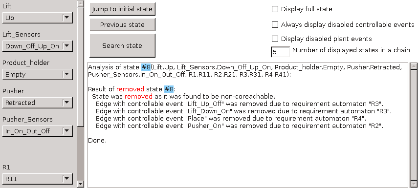
As expected, the analysis tools displays that the state was removed, apparently because it was not co-reachable. Again you get the list of removed edges from this state, as an aid to decide which requirement should be checked, if this was not expected.
The final screenshot shows what is displayed if a state is removed because another state is removed:
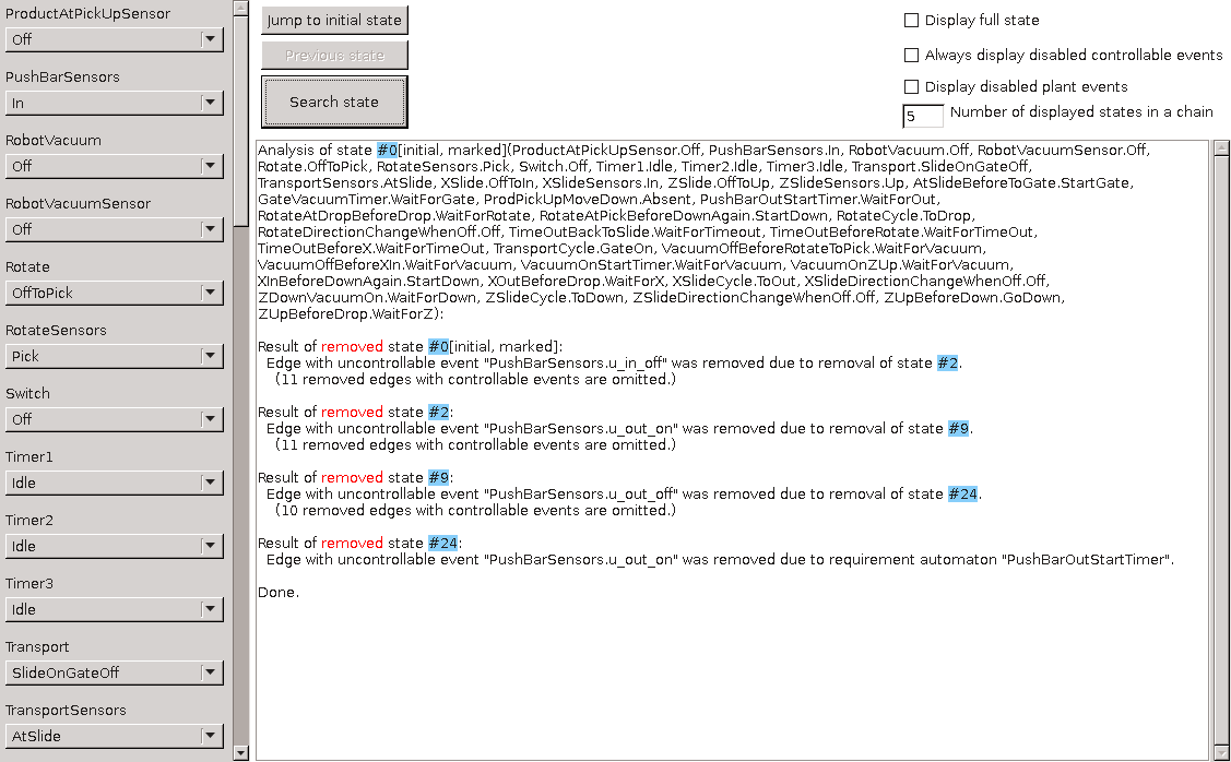
This is an example from a bigger system, where the supervisor is empty. The
analysis of the initial state reveals that it was removed due to a removal of
a chain of other states. State #24 was removed due to a requirement
(reading from bottom to top), which caused the chain of states #9, #2,
and eventually #0 to be removed.
Removed edges with controllable events are not displayed here, since these have no influence to the disappearing of the states. If you want, you can display them by toggling the Always display disabled controllable events option at the top-right.
In this example, the number of states in the chain to the disabling
requirement was 4 states. This chain can be longer. Usually the middle part
is not that interesting and it is omitted from the display, but if you want to
see them, you can increase the number of displayed states at the top-right
(which is by default 5).
Another way to see them is to double-click at a state in the chain, and the
analysis tool will display the chain starting from that state.
A situation that is not shown here, is that the analysis tool has no information about a state. It happens when the synthesis encountered a bad state on all paths to that state. In such a case, it displays that there is no information about the queried state.
Starting the synthesis analysis tool
The tool can be started in the following ways:
-
In Eclipse, double-click a
.synth_dumpfile generated by the supervisor synthesis dump. -
In Eclipse, right click a
.synth_dumpfile in the 'Project Explorer' tab or 'Package Explorer' tab and choose Analyze Synthesis Result. -
Use the
cifsynthanalystool in a ToolDef script. See the scripting documentation and tools overview page for details. -
Use the
cifsynthanalyscommand line tool.
Options
Besides the general application options, this application has the following options:
-
Input file: The absolute or relative local file system path to the input Synthesis dump file.
Event-based nonconflicting check
The nonconflicting check verifies whether two or more automata are conflicting, that is, whether they together could result in non-coreachable states.
One practical application is to check a supervisor, either synthesized or manually created, against a plant. That is, when the supervisor is used to control the plant, will it always stay in the safe coreachable area? If not, at what point does it fail to do so?
Another practical application is to check several supervisors synthesized for parts of a system. That is, when the supervisors are used together to control a system, could that result in non-coreachable states? If so, which states are conflicting?
The tool takes a .cif file containing two or more automata, that must be
both deterministic and trim. Besides those restrictions, the general
event-based restrictions listed at
Supported specifications apply as well.
The nonconflicting check tool produces a text file, listing the traces that lead to a conflicting state. If no such traces are found, the automata are nonconflicting.
Starting the nonconflicting check tool
The tool can be started in the following ways:
-
In Eclipse, right click a
.ciffile in the 'Project Explorer' tab or 'Package Explorer' tab and choose . -
In Eclipse, right click an open text editor for a
.ciffile and choose . -
Use the
cifncchktool in a ToolDef script. See the scripting documentation and tools overview page for details. -
Use the
cifncchkcommand line tool.
Options
Besides the general application options, this application has the following options:
-
Input file: The absolute or relative local file system path to the input CIF specification.
-
Report file: The absolute or relative local file system path to the output report file with conflicts. If not specified, defaults to the input file path, where the
.ciffile extension is removed (if present), and a_conflicts.txtfile extension is added.
Event-based controllability check
The controllability check verifies whether a supervisor automaton does not disable edges with uncontrollable events of the (combined) plant automata. If the check fails, the tool reports where it fails. If the check succeeds, it reports the edges with controllable events that are disabled by the supervisor.
The tool takes a .cif file containing a supervisor automaton, and one
or more plant automata. Besides the general event-based restrictions listed
at Supported specifications, the current implementation
does not support:
-
Having more than one
supervisorautomaton. -
Having no
plantorsupervisorautomaton. -
Having an automaton with a different kind than
plantorsupervisor. -
Having a non-deterministic automaton.
-
Events that are not controllable or uncontrollable, if used (present in the alphabet or on an edge of at least one automaton).
The controllability check tool produces a report text file with its findings. It states whether the controllability property holds (no edges with uncontrollable events of the plant are disabled) or fails (one or more edges with uncontrollable events in the plant are disabled by the supervisor).
If the controllability property holds, the tool lists the disabled controllable events, which can be useful in the design process. If the property fails, the tool lists the edges that are disabled by the supervisor.
Starting the controllability check tool
The tool can be started in the following ways:
-
In Eclipse, right click a
.ciffile in the 'Project Explorer' tab or 'Package Explorer' tab and choose . -
In Eclipse, right click an open text editor for a
.ciffile and choose . -
Use the
cifctrlchktool in a ToolDef script. See the scripting documentation and tools overview page for details. -
Use the
cifctrlchkcommand line tool.
Options
Besides the general application options, this application has the following options:
-
Input file: The absolute or relative local file system path to the input CIF specification.
-
Report file: The absolute or relative local file system path to the output report file with disabled events. If not specified, defaults to the input file path, where the
.ciffile extension is removed (if present), and a_disableds.txtfile extension is added.
Event-based language equivalence check
The language equivalence check verifies whether two automata produce the same language, that is, at every point they are marked in the same way and can produce the same events. Note that even automata with a different number of locations or edges can be language equivalent.
All reachable locations of the automata are checked. In particular, it also checks locations that are outside the marked behavior (that is, reachable locations that are not marked and are not on a path to a marked location). To avoid false positives, you may want to ensure that both automata are trim.
One practical application is to verify whether a manually created supervisor is equivalent to an automatically generated one. If they are not, a counter example is produced.
The tool takes a .cif file containing exactly two automata, that must
be deterministic, have the same alphabet, and have an initial location. In
addition, the general event-based restrictions listed at
Supported specifications apply as well.
The language equivalence check tool produces output stating
Automata have the same language, or it produces a counter example
where an event can be
performed in a location in one automaton, while from the equivalent
location in the other automaton the same event cannot be performed.
The equivalent location is derived by walking from the initial
location to the location of interest in both automata, using the same
sequence of events.
Starting the language equivalence check tool
The tool can be started in the following ways:
-
In Eclipse, right click a
.ciffile in the 'Project Explorer' tab or 'Package Explorer' tab and choose . -
In Eclipse, right click an open text editor for a
.ciffile and choose . -
Use the
ciflngeqvtool in a ToolDef script. See the scripting documentation and tools overview page for details. -
Use the
ciflngeqvcommand line tool.
Options
Besides the general application options, this application has the following options:
-
Input file: The absolute or relative local file system path to the input CIF specification.
Event-based NFA to DFA automaton conversion
The event-based NFA to DFA automaton conversion takes an non-deterministic automaton. The algorithm produces a deterministic automaton with the same language.
The tool takes a .cif file containing a single automaton. The output is
a .cif file containing a deterministic automaton that is language
equivalent with the input automaton. The resulting automaton has the same kind
as the input automaton.
Starting the NFA to DFA automaton conversion tool
The tool can be started in the following ways:
-
In Eclipse, right click a
.ciffile in the 'Project Explorer' tab or 'Package Explorer' tab and choose . -
In Eclipse, right click an open text editor for a
.ciffile and choose . -
Use the
cifnfadfatool in a ToolDef script. See the scripting documentation and tools overview page for details. -
Use the
cifnfadfacommand line tool.
Options
Besides the general application options, this application has the following options:
-
Input file: The absolute or relative local file system path to the input CIF specification.
-
Output file: The absolute or relative local file system path to the output CIF specification. If not specified, defaults to the input file path, where the
.ciffile extension is removed (if present), and a_dfa.ciffile extension is added. Thedfapart of the default extension depends on the Result name option. -
Result name: The name to use for the projected automaton. If not specified, defaults to
dfa. Also affects the Output file option.
Event-based DFA minimization
Minimizing the number of locations of an automaton while preserving the language gives a canonical representation of the language, making it easier to compare automata. The DFA minimization tool computes such a minimal automaton.
The tool takes a .cif file containing one deterministic automaton with an
initial location. In addition, the general event-based restrictions listed at
Supported specifications apply as well.
The DFA minimization tool produces an automaton with the same language, but with the minimal number of locations. If the original automaton already had the minimal number of locations, the result is the same as the input.
Starting the DFA minimization tool
The tool can be started in the following ways:
-
In Eclipse, right click a
.ciffile in the 'Project Explorer' tab or 'Package Explorer' tab and choose . -
In Eclipse, right click an open text editor for a
.ciffile and choose . -
Use the
cifdfamintool in a ToolDef script. See the scripting documentation and tools overview page for details. -
Use the
cifdfamincommand line tool.
Options
Besides the general application options, this application has the following options:
-
Input file: The absolute or relative local file system path to the input CIF specification.
-
Output file: The absolute or relative local file system path to the output CIF specification. If not specified, defaults to the input file path, where the
.ciffile extension is removed (if present), and a_minimal.ciffile extension is added. Theminimalpart of the default extension depends on the Result name option. -
Result name: The name to use for the minimized automaton. If not specified, defaults to
minimal. Also affects the Output file option.
Event-based automaton projection
The event-based automaton projection takes an automaton and a subset of the
events of its alphabet that should be preserved. The other events of the
alphabet are considered to be internal steps and get replaced by epsilon
at the edges. The algorithm produces a deterministic automaton with the subset
as its alphabet that has the same language.
The tool takes a .cif file containing a single automaton, and the names
of the events that should be preserved. The output is a .cif file
containing a deterministic automaton that is language equivalent with the
input automaton with respect to the set of preserved events.
The resulting automaton has the same kind as the input automaton.
Starting the automaton projection tool
The tool can be started in the following ways:
-
In Eclipse, right click a
.ciffile in the 'Project Explorer' tab or 'Package Explorer' tab and choose . -
In Eclipse, right click an open text editor for a
.ciffile and choose . -
Use the
cifprojtool in a ToolDef script. See the scripting documentation and tools overview page for details. -
Use the
cifprojcommand line tool.
Options
Besides the general application options, this application has the following options:
-
Input file: The absolute or relative local file system path to the input CIF specification.
-
Preserved events: Comma and/or whitespace separated absolute names of events that should be preserved.
-
Output file: The absolute or relative local file system path to the output CIF specification. If not specified, defaults to the input file path, where the
.ciffile extension is removed (if present), and a_projected.ciffile extension is added. Theprojectedpart of the default extension depends on the Result name option. -
Result name: The name to use for the projected automaton. If not specified, defaults to
projected. Also affects the Output file option.
Event-based observer check
The event-based observer check takes an automaton, and a subset of the events of its alphabet that are observable. The check verifies whether the automaton after projection (see Event-based automaton projection) can derive the (abstracted) state of another component by synchronizing only on the observable events.
The tool takes a .cif file containing a single automaton, and the names
of the events that are observable. The output is a report file that indicates
whether the observer check property holds. If it fails, the events causing
failure are also listed.
Starting the observer check tool
The tool can be started in the following ways:
-
In Eclipse, right click a
.ciffile in the 'Project Explorer' tab or 'Package Explorer' tab and choose . -
In Eclipse, right click an open text editor for a
.ciffile and choose . -
Use the
cifobschktool in a ToolDef script. See the scripting documentation and tools overview page for details. -
Use the
cifobschkcommand line tool.
Options
Besides the general application options, this application has the following options:
-
Input file: The absolute or relative local file system path to the input CIF specification.
-
Observable events: Comma and/or whitespace separated absolute names of events that are observable.
-
Report file: The absolute or relative local file system path to the output report file. If not specified, defaults to the input file path, where the
.ciffile extension is removed (if present), and a_observation.txtfile extension is added.
Event-based automaton abstraction
The event-based automaton abstraction takes an automaton, and a subset of the events of its alphabet that are observable. The abstraction produces a non-deterministic abstracted automaton with the observable events as its alphabet, that is weakly bisimilar to the original automaton.
The tool takes a .cif file containing a single automaton, and the names
of the events that are observable. The output is a .cif file with the
abstracted automaton. The resulting automaton has the same kind as the input
automaton.
Starting the automaton abstraction tool
The tool can be started in the following ways:
-
In Eclipse, right click a
.ciffile in the 'Project Explorer' tab or 'Package Explorer' tab and choose . -
In Eclipse, right click an open text editor for a
.ciffile and choose . -
Use the
cifabstrtool in a ToolDef script. See the scripting documentation and tools overview page for details. -
Use the
cifabstrcommand line tool.
Options
Besides the general application options, this application has the following options:
-
Input file: The absolute or relative local file system path to the input CIF specification.
-
Observable events: Comma and/or whitespace separated absolute names of events that are observable.
-
Output file: The absolute or relative local file system path to the output CIF file. If not specified, defaults to the input file path, where the
.ciffile extension is removed (if present), and a_abstracted.ciffile extension is added. Theabstractedpart of the default extension depends on the Result name option. -
Result name: The name to use for the abstracted automaton. If not specified, defaults to
abstracted. Also affects the Output file option.
Event-based trim check
This check verifies that the automata in the given file are trim, that is, in each automaton, all the locations must be both reachable and coreachable. If the check fails for one or more automata, the tool reports for each automaton, whether all its locations are reachable and coreachable. It also lists the locations where the property fails.
Starting the trim check tool
The tool can be started in the following ways:
-
In Eclipse, right click a
.ciffile in the 'Project Explorer' tab or 'Package Explorer' tab and choose . -
In Eclipse, right click an open text editor for a
.ciffile and choose . -
Use the
ciftrimchktool in a ToolDef script. See the scripting documentation and tools overview page for details. -
Use the
ciftrimchkcommand line tool.
Options
Besides the general application options, this application has the following options:
-
Input file: The absolute or relative local file system path to the input CIF specification.
-
Report file: The absolute or relative local file system path to the output report file with disabled events. If not specified, defaults to the input file path, where the
.ciffile extension is removed (if present), and a_trimcheck.txtfile extension is added.
Event-based trim
The trim tool makes an automaton trim by removing all locations that are not
reachable or coreachable.
The input is a .cif file with a single automaton, and the tool produces a
new .cif file with the trim automaton. If the automaton in the input was
already trim, all locations are preserved.
Starting the trim tool
The tool can be started in the following ways:
-
In Eclipse, right click a
.ciffile in the 'Project Explorer' tab or 'Package Explorer' tab and choose . -
In Eclipse, right click an open text editor for a
.ciffile and choose . -
Use the
ciftrimtool in a ToolDef script. See the scripting documentation and tools overview page for details. -
Use the
ciftrimcommand line tool.
Options
Besides the general application options, this application has the following options:
-
Input file: The absolute or relative local file system path to the input CIF specification.
-
Output file: The absolute or relative local file system path to the output CIF specification. If not specified, defaults to the input file path, where the
.ciffile extension is removed (if present), and a_trim.ciffile extension is added. Thetrimpart of the default extension depends on the Result name option. -
Result name: The name to use for the trim automaton. If not specified, defaults to
trim. Also affects the Output file option.
CIF to Supremica transformer
The CIF to Supremica transformer can be used to transform CIF specifications
to Supremica modules (*.wmod files).
Supremica
is a tool for synthesis of discrete event supervisors.
Starting the transformation
The transformation can be started in the following ways:
-
In Eclipse, right click a
.ciffile in the 'Project Explorer' tab or 'Package Explorer' tab and choose . -
In Eclipse, right click an open text editor for a
.ciffile and choose . -
Use the
cif2supremicatool in a ToolDef script. See the scripting documentation and tools overview page for details. -
Use the
cif2supremicacommand line tool.
Options
Besides the general application options, this application has the following options:
-
Input file path: The absolute or relative local file system path to the input CIF specification.
-
Output file path: The absolute or relative local file system path to the output Supremica module file. If not specified, defaults to the input file path, where the
.ciffile extension is removed (if present), and a.wmodfile extension is added. -
Supremica module name: The name of the Supremica module. If not specified, defaults to the name of the output file, after removal of the
.wmodextension (if present). -
Eliminate enumerations: Enable this option to eliminate enumerations before generating transforming to Supremica. Disable this option to keep enumerations in the generated Supremica module. By default this option is disabled.
Even though Supremica supports enumerations in its language, it doesn’t support them in all its algorithms. Even if the original CIF transformation being transformed does not use enumerations, enumerations may still be generated internally during preprocessing.
Supported specifications
The CIF to Supremica transformer supports a subset of CIF specifications. The following restrictions apply:
-
Kindless/regular automata (without a supervisory kind) are not supported. Only
plant,requirement, andsupervisorautomata are supported. -
Events not declared as controllable or uncontrollable are not supported. This includes the
tauevent, both explicitly used on edges, as well as implicitly for edges without explicitly mentioned events. -
Initialization predicates outside of locations are not supported.
-
Marker predicates outside of locations are only supported if they have the form
discrete_variable = marked_value. -
Discrete variables with multiple marker predicates are not supported.
-
Locations with initialization or marker predicates that are not trivially true or false are not supported.
-
Automata that do not have exactly one initial location are not supported.
-
Invariants in locations are not supported.
-
Invariants are only supported if they are requirement invariants.
-
Only state invariants are supported. State/event exclusion invariants are not supported. To allow state/event exclusion invariants to be used in the input, manually eliminate them first using the Eliminate state/event exclusion invariants CIF to CIF transformation.
-
Discrete variables that have multiple potential initial values (
in {...}orin any) are not supported. -
Continuous variables are not supported.
-
Input variables are currently unsupported.
-
Multi-assignments on edges (such as
do (x, y) := (1, 2)) are not supported. However, it is allowed to use multiple assignments on an edge (such asdo x := 1, y := 2). -
Partial variable assignments (such as
do x[0] := 5) are not supported. -
Conditional updates on edges (such as
do if b: x := 5 end) are not supported. -
Urgent locations and urgent edges are not supported.
-
User-defined functions are not supported.
-
Channels (events with data types) are not supported.
-
Only the following data types are supported: boolean types, ranged integer types, and enumeration types.
-
Only the following expressions are supported: boolean literal values, integer literal values, binary expressions (partially, see below), unary expressions (partially, see below), and references to constants, discrete variables, enumeration literals, and casts that don’t change the type.
-
Only the following binary operators are supported: logical equivalence (
<=>), logical implication (=>), conjunction (and) on boolean operands, disjunction (or) on boolean operands, addition (+) on ranged integer operands, subtraction (-) on ranged integer operands, multiplication (*) on ranged integer operands, integer division (div) on ranged integer operands, integer modulus (mod) on ranged integer operands, equality (=), inequality (!=), less than (<) on ranged integer operands, less than or equal to (<=) on ranged integer operands, greater than (>) on ranged integer operands, and greater than or equal to (>=) on ranged integer operands. -
Only the following unary operators are supported: logical inverse (
not), negation (-) on a ranged integer operand, and plus (+) on a ranged integer operand.
Preprocessing
The following CIF to CIF transformations are applied as preprocessing (in the given order), to increase the subset of CIF specifications that can be transformed:
-
Eliminate enumerations (if enabled via the corresponding option)
Transformation result
The CIF automata kinds plant, requirement, and supervisor are
mapped to Supremica kinds Plant, Specification, and Supervisor,
respectively.
All generated Supremica automata are tagged as non-deterministic, as CIF automata may be non-deterministic.
Nameless CIF locations are given the name X in Supremica automata.
Supremica does not support boolean values. Instead of true, value 1 is
used, and instead of false, value 0 is used. For boolean types
(bool), ranged integer types (int[0..1]) are used.
The absolute names of all CIF objects (automata, variables, etc) are used,
where the . characters are replaced by : characters. For enumeration
literals, the non-absolute name of the enumeration literal is used, prefixed
with :lit:.
No geometry is generated. When the generated Supremica file is opened in Supremica, Supremica will perform auto layouting.
Initialization
For the initial values of the variables, initialization predicates are
generated (e.g. x == 3). Earlier versions of Supremica that support
variables allowed deterministic initialization (only the initial value), and
non-deterministic initialization (initialization predicates). The most recent
version only allows non-deterministic initialization, which is why we generate
initialization predicates.
Marking
In CIF, if none of the locations of an automaton are indicated as marked, the
automaton has no marked locations. In Supremica, if none of the locations of
an automaton are indicated as marked (:accepting), all locations of the
automaton are implicitly marked. When transforming a CIF automaton without any
marked locations, a warning is printed to the console to inform the user of
this difference.
In CIF, if none of the values of a variable is indicated as marked, the
variable has no marked values. In Supremica, if none of the values of
a variable is indicated as marked (:accepting), all values of the
variable are implicitly marked. When transforming a CIF variable without any
marked values, a warning is printed to the console to inform the user of
this difference.
Location pointer variables that are automatically generated, such as the ones generated by the Eliminate the use of locations in expressions CIF to CIF transformation, have no marking and thus lead to warnings.
Invariants
If the CIF model being transformed contains state invariants, an uncontrollable
u_inv_bad event is added to the Supremica module. It is renamed if the name
is not unique. A plant automaton named inv_plant (renamed if not unique) is
added as well. This plant enables the u_inv_bad event if and only if at
least one of the invariants doesn’t hold. A requirement automaton inv_req
(renamed if not unique) is added as well. The requirement disables the event
globally. Since blocking an uncontrollable plant event in a requirement is
forbidden, synthesis will prevent such blockage (by disabling controllable
events), thereby ensuring that the state invariants hold after synthesis.
Alphabets
In CIF, it is possible to explicitly specify the alphabet of an automaton. This
alphabet may include more events than occur on the edges of the automaton,
thereby globally disabling those additional events. Supremica automatically
determines the alphabet automatically, based on the events that occur on the
edges of the automaton, just like CIF does if no explicit alphabet is
specified. If a CIF automaton with 'additional' events is transformed, a self
loop is added to the initial state for each 'additional' event, with a
false guard (0 in Supremica). This ensures that the event occurs on
an edge, and is thus part of the alphabet, but is not enabled.
Range semantics
In CIF, if an update of an edge results in out of range values of variables, the CIF specification is considered invalid, and the simulation will result in a runtime error. In Supremica, the simulation does not result in a runtime error, but instead the offending transition is disabled/forbidden.
Jumping semantics
Consider the following CIF model:
plant automaton p:
  controllable c_event;
  disc int[0..3] v = 0;

  location loc1:
    initial;
    marked;
    edge c_event do v := v + 1 goto loc2;

  location loc2:
    edge c_event               goto loc1;
end
There are two locations, and the edges allow for moving from one location to
the other. Both edges use the same event. Every odd transition (the first
transition, the third transition, etc), the value of variable v is
increased by one. Every even transition, the value of variable v is not
changed. After a few transitions, the simulation crashes due to overflow of
variable v.
To ensure the same semantics in Supremica, such that for every even transition
the value of variable v does not change, the CIF model is modified by the
transformation, to the following:
plant automaton p:
  controllable c_event;
  disc int[0..3] v = 0;

  location loc1:
    initial;
    marked;
    edge c_event do v := v + 1 goto loc2;

  location loc2:
    edge c_event do v := v     goto loc1;
end
Users of the transformation don’t have to do anything themselves, as the tool
automatically adds the dummy assignments as needed. If the tool would not have
added such dummy assignments, then the value of variable v would have
been able to jump to any value (in its range [0..3]) for every even
transition, according to the Supremica semantics.
Simulation, validation, and visualization tools
CIF simulator
The CIF simulator can be used to explore the state space of CIF specifications, either interactively, or using a more automated approach. Powerful visualization features allow for interactive visualization-based validation of the CIF specification.
Basics
Input/Output
-
Environment events (non-urgent events)
Advanced
-
ODE solver (integration and guard/event detection)
Miscellaneous
Developers
Simulation basics
Supported specifications
The CIF simulator supports a subset of CIF specifications. The following restrictions apply:
-
Input variables are currently not supported.
-
Time dependent state invariants are not supported. This applies only to state invariants. State/event exclusion invariants are supported.
Specifications with component definitions/instantiations are not natively supported by the CIF simulator. Therefore, they are automatically eliminated by the simulator, as a preprocessing step, using the CIF to CIF transformation to eliminate component definition/instantiation.
Automata with multiple possible initial locations and discrete variables with
multiple possible initial values (including any) are not supported, unless
additional initialization is provided.
The controllability of events is ignored by the simulator, as are marker predicates.
All automata are simulated as plants. That is, all automaton kinds are ignored by the simulator. However, simulating requirements as plants may lead to unexpected results. Therefore, the simulator prints warnings to the console, whenever requirements are simulated. It is highly recommended to first apply supervisor synthesis to the specification, and simulate the resulting specification using the simulator. Alternatively, apply verification to the specification, remove the verified requirements, and simulate the resulting specification using the simulator.
Similar to requirement automata, the simulator warns about simulation of requirement invariants.
Starting the simulator
The CIF simulator can be started in the following ways:
-
In Eclipse, right click a
.ciffile in the 'Project Explorer' tab or 'Package Explorer' tab and choose Simulate CIF specification…. -
In Eclipse, right click an open text editor for a
.ciffile and choose Simulate CIF specification…. -
Use the
cifsimtool in a ToolDef script. See the scripting documentation and tools overview page for details. -
Use the
cifsimcommand line tool.
Once you start the simulator, an option dialog will appear, where you can configure the simulation options.
Instead of a CIF model (e.g. a .cif file), simulation can also be started
for a compiled code file (e.g. a
.cifcode file). For compiled code files, an additional option is
available. The simulator can also be started by double clicking such a file.
Initialization of the CIF specification
CIF supports discrete variables with multiple potential initial values, as well as discrete variables with an arbitrary initial value. Furthermore, CIF supports automata with multiple potential initial locations. The simulator however, needs to know how to initialize the specification. The initial values of discrete variables, and the initial locations of automata, can be specified using the CIF specification initialization option (Simulator category). Initialization can be provided using the option, per discrete variable or automaton.
For a discrete variable, initialization is of the form var:value, where
var is the absolute name of a discrete variable, and value is a CIF
literal that represents a
valid initial value for the variable. Providing an initialization for a
discrete variable with a
function type or a
distribution type, is not supported.
For an automaton, initialization is of the form aut:loc, where aut is
the absolute name of an automaton, and loc is the name of a location of
that automaton. Providing an initialization for an automata with only one
nameless location, is not supported.
It is not allowed to provide multiple initializations for a single variable or automaton.
If insufficient initializations are provided, variables and automata may not be initialized. That is, the simulator may not be able to choose between the multiple potential initial values or locations. The simulator will report such problems, indicating the specification is unsupported without additional or alternative initializations.
It is also possible that initializations in the CIF specification itself are incomplete or conflicting, the provided initializations are conflicting, or their combination is conflicting. Furthermore, initializations may be provided for values or locations that are not potential initial values or locations. In all such cases, initialization fails. The simulator will report such problems, providing detailed information about what caused the initialization failure.
Terminating the simulator
The CIF simulator can terminate for various reasons. This page explains each of them, as well as some other information related to termination of the simulator.
Initialization failure
If initialization of the specification fails, the simulation will terminate immediately.
Deadlock
If simulation results in deadlock, no more transitions are possible, and the simulation will terminate.
Simulation does not immediately terminate when deadlock occurs, if an interactive input mode is used and history is enabled. Instead, the user is asked whether to terminate the simulation, undo one or more transitions, or reset the simulation.
Simulation end time
Using the
Simulation end time
option (Simulator
category), the end time of the simulation can be configured. By setting a
simulation end time, you ensure that when the value of variable time
reaches that value, the simulation terminates.
By default the simulation end time is set to 'infinite', which means that simulation termination is not limited by a simulation end time. Settings a simulation end time also limits the maximum duration of a time transition.
Simulation does not immediately terminate when the configured end time is reached, if an interactive input mode is used and history is enabled. Instead, the user is asked whether to terminate the simulation, undo one or more transitions, or reset the simulation.
Runtime error
If simulation results in a runtime error, the simulation will terminate immediately.
End of trace file
If the trace input mode is used, and no more commands are available in the trace file, the simulation will terminate immediately.
User-requested termination
The user can manually request termination of the simulation in several ways.
Termination requests have no effect while the simulator interactively asks for input from the console or via the GUI of the interactive GUI input component. However, once input is provided via the console and ENTER is pressed, or a choice is made via the GUI, the termination request will be processed.
Termination requests issued between intermediate frames are delayed until the next intermediate frame.
Termination of the simulation can be requested, when using the interactive
console input mode, by typing q
and pressing ENTER, whenever the simulator interactively asks for input
via the console.
Termination of the simulation can be requested, when using the interactive interactive GUI input mode, by closing the GUI of the interactive GUI input component, when the simulator asks for input via that GUI.
The Applications view has several termination features that may terminate any application, including the CIF simulator. See the documentation for that view, for details.
Simulation can be terminated at any time, by using the Terminate
button ( ), located at the upper right corner of the console.
Note however that if the console does not have the focus, this button may not be visible. If the button is not visible, click somewhere in the console to make the button appear. If even then the button is still not available, it may still appear if you Maximize the console. Due to these issues, use of the termination features of the Applications view is recommended over using the Terminate button of the console. See the documentation for that view, for details.
If the last remaining real-time output component (visualizer) is closed by the user, the simulator will be asked to terminate as soon as possible.
Confirming termination
When simulating within Eclipse, all visualizers remain open, after the simulation has terminated. This allows you to observe the final state of the simulation, before manually closing the visualizers.
When simulating on the command line (outside of Eclipse), termination of the simulator means that the visualizers are also closed. To allow you to observe the final state of the simulation, you are asked to confirm termination of the simulator, and therefore closing of the visualizers, by pressing ENTER at the console.
By default, you are only asked to confirm termination of the simulator when simulating on the command line (outside of Eclipse), at least one visualizer is visible at the end of the simulation, simulation did not result in a runtime error, and test mode is disabled. The Ask to confirm simulator termination option (Simulator category) can be used to configure whether the simulator asks the user to confirm termination of the simulator, terminate automatically, or decides by itself whether to ask the user for confirmation or terminate automatically. The latter (letting the simulator decide by itself) is the default.
Simulation of traces
The CIF simulator simulates one particular trace through the state space of the specification. To better understand what the previous sentence means, this page further explains each of those concepts.
State
Automata consist of one or more locations. However, at any time, an automaton can only be in one of its locations. This location is called the current or active location. The current location of an automaton is also called the state of the automaton.
Similar to having multiple locations in automata, variables usually have many possible values. However, similar to automata having only one current location, variables can not have two values at the same time.
The current location of each of the automata (i.e. the states of the automata),
together with the current values of the variables (all discrete and continuous
variables, including variable time), is called the state of the
specification. The state of the specification (or simply 'the state'), is
all the information that needs to be maintained about the history of the
simulation, going forward.
For instance, consider the following specification:
automaton button:
event pushed, released;
location Released:
initial;
edge pushed goto Pushed;
location Pushed:
edge released goto Released;
end
automaton machine:
event producing, produced;
location Idle:
initial;
edge producing when button.Pushed goto Producing;
location Producing:
edge produced goto Idle;
endWe have two automata, button and machine. Pushing the button (event
button.pushed) turns on the machine. Releasing the button (event
button.released) turns it off. Initially, the machine is Idle. While
the button is pushed (location button.Pushed is the current location of
automaton button), the machine can start to create a product (event
machine.producing). Once the machine has produced a product (event
machine.produced), the machine becomes idle again. Note that once the
machine starts producing a product, it always finishes producing it, even if it
is turned off in the mean time.
The state of automaton button is either of its locations:
button.Released or button.Pushed. Similarly, the state of automaton
machine is machine.Idle or machine.Producing. Initially, the system
is in state button: Released, machine: Idle, time: 0.0. For the remainder of
variable time will omitted from the state, for brevity only. Furthermore,
also for brevity only, we’ll omit the names of the automata. Therefore, the
initial state is Released, Idle.
State space
The state space of a specification consists all the possible states of the specification, connected by the transitions via which they can be reached.
For the example above, the state space is (event names are abbreviated):
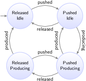
Since both automata can be in two states, the state space in this case consists of four states. From the initial state (the upper left state), the button can be pushed, leading to the upper right state, where the button is pushed, while the machine has not yet started to produce a product. The machine can then start to produce a product (going to the lower right state). If however the button is released before the machine can respond by starting to produce a product, we go back to the upper left state. When the machine finishes creation of the product, we go from the lower right state back to the upper right state. If on the other hand the button is released, while the product is still being produced, we go from the lower right state to the lower left state. If we then push the button again, we go back to the lower right state. If instead the button is not pushed, and the machine finishes producing the product, we go from the lower left state back to the upper left state.
Traces
A trace is a sequence of transitions, from the initial state, through the state space.
In state spaces, most states usually have multiple outgoing transitions. This means there is choice. That is, it is possible to choose to which next state to go. Furthermore, it is usually possible to keep taking transitions forever, which means we can have infinite traces.
For the example above, some of the possible traces are shown below. Only the first five transitions of the traces are shown. State names are abbreviated, to the first letters of the names of the locations.
-
RI →
pushed→ PI →released→ RI →pushed→ PI →released→ RI →pushed→ PI → … -
RI →
pushed→ PI →producing→ PP →produced→ PI →producing→ PP →produced→ PI → … -
RI →
pushed→ PI →producing→ PP →released→ RP →produced→ RI →pushed→ PI → …
In the first trace, we push the button, release it, push it again, release it, and push it again, all without ever starting to produce a product. This traces shows us what happens if the button is constantly being pushed and released, as quickly as possible, without the machine being able to respond to this, by starting to produce a product.
In the second trace, we push the button, we start to produce a product, we finish producing it, start to produce another product (the button is still pushed), finish producing the second product, and start to produce a third product. This is a trace of a typical usage scenario, where we start the machine, and the machine keeps running.
In the third trace, we push the button, start to produce a product, release the button before the product is finished, finish producing the product, and push the button again. This trace is another typical usage scenario, which also includes turning off the machine.
Simulation
As stated at the top of the page: 'The CIF simulator simulates one particular trace through the state space of the specification'. To see why this is the case, we take a look at the main simulation loop, as used by the simulator:
-
Calculate the initial state, and set it as the current state.
-
Forever, do:
-
If the user-provided simulation end time is reached, stop simulation.
-
Calculate the possible transitions for the current state.
-
If no transitions are possible (deadlock), stop simulation.
-
Choose one of the possible transitions.
-
Take the chosen transition, and set its target state as the new current state.
-
While this main simulation loop is simplified with respect to the real implementation, it gives some insight into the inner workings of the simulator. The simulator keeps taking transitions. Once a transition is taken, the current state is updated to the target state of the transition. This means that the other possible transitions (the ones that were not chosen), are not taken. Therefore, if we want to take a different transition, we should restart simulation from the initial state, and make different choices. That is, if we want to simulate a different trace, we perform another simulation.
Validation
The simulator can be used to gain confidence in the correctness of the specification. By simulating various traces, we can observe what happens in different scenarios (use cases). Since the number of traces if often infinite, covering the entire state space, and all possible traces, is impossible. However, by wisely choosing the traces we simulate, we can cover a large part of the state space.
It should be clear by now, that simulating a single trace is almost never enough to conclude that your specification is 'correct'. Different traces lead to different behavior, and only by testing enough traces, and thus covering enough of the system’s behavior, can you conclude that your specification works as expected (for those traces).
Repeated simulation
When simulating a CIF model, the simulator reads the CIF file, checks it for validity, generates Java code, compiles the code, and uses the compiled code using the actual simulation. All of this takes a bit of time, or even quite some time, depending on the size of the model. This situation is not ideal for repeated simulations, for instance when trying different scenarios or use cases, when simulating with different options, or when repeating simulations with various different initializations or due to stochastic behavior. The startup time for the first simulation is also present for the second simulation, etc.
It would be much better to generate and compile the code just once, and then simulate multiple times using the already compiled code, significantly reducing the startup time of the simulations. This is especially useful for automated repeated simulations, where the same simulation model, either with different options (for instance different initializations) or with the same options for a model with stochastics, is simulated multiple times and the results of simulation are for instance compared or aggregated in some way.
Compiling just once
The simulator can be used to generate code and compile it only once. By enabling the Compile only option (Compiler category), the simulator will perform all steps needed to generate and compile the code, and will then save the compiled code to a file. After saving the file, the simulator will terminate, not simulating the model.
By default, the input file name (e.g. some_file.cif) is used to construct
the name of the simulator compiled Java code file, by removing the .cif
file extension if present, and adding a .cifcode file extension to it (e.g.
resulting in some_file.cifcode). It is possible to change this file name
by using the Compiled code file option (Compiler category). If used, it
specifies the absolute or relative local file system path to the compiled Java
code file.
The compiled code file can be put in any directory. It does not have to be in the same directory as the original CIF model. However, make sure that any additional files, such as SVG images for visualization, remain in their original locations. They will be resolved relative to the original location of the CIF model that was compiled.
Simulating using a compiled code file
There are several ways to start simulation with a compiled code file. In fact,
all the ways to start simulation for normal CIF
models (e.g. .cif files), apply to compiled code files (e.g. .cifcode
file) as well. The simulator checks whether the input file name ends with
.cifcode and then loads the compiled code file, instead of treating the
input model as CIF model.
Alternatively, a .cifcode file can be double clicked in the Eclipse
'Project Explorer' tab or 'Package Explorer' tab, to immediately
start simulation. An option dialog is shown to configure any simulator
options.
A warning is printed to the console if the compiled code file was generated by a different version of the simulator than the one used to simulate it. Ignoring the warning may lead to unexpected simulation results, or even simulator crashes.
Option effects and priorities
Most simulator options have no effect when the Compile only option (Compiler category) is enabled, as after code is generated, compiled, and saved to a file, the simulator terminates, and no actual simulation is performed.
The Compile only option (Compiler category) has no effect when debugging generated code, by enabling the Load debug code option (Simulator category).
Example
As an example, consider the following CIF model in file machine.cif:
event enter;
event processed;
event exit;
automaton machine:
disc int count = 0;
disc real process_time;
disc dist real d = normal(10, 7);
cont t der 1.0;
location waiting:
initial;
edge enter do (process_time, d) := sample d, t := 0 goto processing;
location processing:
edge processed when t >= process_time goto done;
location done:
edge exit do count := count + 1 goto waiting;
end
print machine.count for final;The model consists of a machine that processes products. Initially, the
machine is waiting. Once a product enters the system, the machine will
start processing. Once the product is processed, the machine is
done and will be waiting for the next product to enter. The time it
takes to process a product varies with each product. A
normal distribution
with
a mean of 10 and a variance of 7 is used to model the varying
processing times.
The print declaration at the end of the model is used to print the number of processed products at the end of the simulation.
Consider the following ToolDef script:
from "lib:cif" import *;
cifsim("machine.cif --compile-only=on");
rmfile("out.txt", force=true);
for x in range(1000):
string args = "machine.cifcode -i auto -a first -t 100 -o print";
cifsim(args, stdout="out.txt", appendOut=true);
end
double minimum = 9999;
double maximum = -9999;
for line in readlines("out.txt"):
double value = <double>line;
minimum = min(minimum, value);
maximum = max(maximum, value);
end
outln("Minimum: %.2f", minimum);
outln("Maximum: %.2f", maximum);The import statement makes the CIF tools available. The first cifsim
command generates code for the machine.cif model, compiles it, and saves it
to machine.cifcode. The rmfile command removes the out.txt file, in
case it was left over from a previous run of the script.
The body of the for statement is executed 1000 times. Each time, the
cifsim command is used to simulate the model, using the already compiled
code in machine.cifcode. The simulation uses
automatic mode due to -i auto,
always chooses the first available
transition due to -a first, ends
at time 100 due to -t 100, and only
outputs text for print declarations due
to -o print. The output of the simulation is not written to the console,
but to out.txt due to the use of the stdout parameter of the
cifsim tool. The appendOut parameter is enabled to ensure that the
output of each simulation is appended (added) to the out.txt file instead
of overwriting the file for each simulation. After the simulations, the
out.txt file will contain the number of processed products for each of the
simulation experiments.
The remainder of the script computes the minimum and maximum number of products
(minimum and maximum throughput) of the machine, as observed from the
experiments. Both the minimum and maximum are initialized. Then each
line of the out.txt file is processed. The numeric value is obtained by
casting the text of the line to a double number. Then the minimum and
maximum are updated as needed. After the minimum and maximum are
calculated, they are printed to the console as floating point numbers with two
digits after the decimal mark.
The output of the execution of the script could look like this, but may vary given that stochastics are used:
Minimum: 7.00
Maximum: 12.00Applications view
The Applications view shows the current status of each running application. For repeated simulation, lots of applications may be started in a short period of time. Also, a lot of status updates need to be processed by the view in a short amount of time. This may lead to many updates of the GUI of the Applications view, which could potentially reduce the responsiveness of Eclipse, and decrease the performance of the simulation. If you experience such problems, simply close the Applications view while running a repeated simulation.
Simulation input/Output
Input modes
The CIF simulator simulates traces through the state space of a specification. If multiple transitions are possible, a choice must be made. The simulator defers this choice to an input component.
The primary responsibility or an input component is to choose the transition to take, from the given possible transitions, calculated for the current state. If the chosen transition is a time transition, the input component must also decide the amount of time to delay.
The input component to use for the simulation, depends on the input mode, which can be configured via the Input mode option (Input category). The simulator has several input modes:
Only one input mode, and thus one input component, can be used for each simulation. By default, the GUI input mode is used.
The following information on other topics, related to input modes, is available:
-
State history (reset, undo)
Interactive console input mode
In the interactive console input mode, the simulator interactively asks the user to choose the transitions to take, etc. The questions are asked via text printed to the console. The user enters his/her choice via the console as well.
The following is an example of the simulator interactively asking the user to choose a possible transition:
Possible transitions:
#1: event machine1.c_start
#2: event machine2.c_start
#3: delay for (0 .. 100.0]
Select a transition ([1..3]). Enter q to quit. Enter h for help and additional commands. Confirm with <ENTER>:Here, three possible transitions are given, numbered 1 to 3. For your
convenience, they are sorted alphabetically on the names of the events, with
event tau always at the end, just before time transitions.
The user should enter a command, and confirm that choice by pressing ENTER. Several command are available:
-
Entering a number in the given range, corresponding to the transition with that number, will result in that specific transition being taken. So, entering
2and pressing ENTER, will result in the simulator taking the transition for eventmachine2.c_start. The valid choices for the transitions are indicated by the range[1..3]. In case of an invalid number, an error message is printed to the console, and the user can choose again. -
Entering nothing, and only pressing ENTER, defaults to choosing transition
1. -
Entering
rorR, and confirming that by pressing ENTER, will reset the simulation to the initial state. If reset is not enabled, or not possible for the current state, an error message is printed and the user can choose again. -
Entering
uorU, and confirming that by pressing ENTER, will undo one transition. If undo is not enabled, or not possible for the current state, an error message is printed and the user can choose again. -
Entering
u <n>orU <n>, with<n>a positive number, and confirming that by pressing ENTER, will undontransitions. If undo is not enabled, it is not possible to undontransitions for the current state, an error message is printed and the user can choose again. -
Entering
qorQ, and confirming that by pressing ENTER, will terminate the simulation. -
Entering
horH, and confirming that by pressing ENTER, will result in the simulator printing a short help text to the console, that shows the available commands. The user is then again asked to choose.
If a choice is made that is invalid or is not available for the current state, an error message is printed to the console, and the user is asked to make an other choice.
If the user chooses a time transition (choice 3 in the above example), the
simulator subsequently asks for the duration of the time delay:
Select a duration from (0 .. 100.0]. Empty choice equals maximum delay. Enter q to quit. Confirm with <ENTER>:Here, the duration of the time delay is to be entered. In this case, the
duration must be in the (0 .. 100.0] interval. That is, it must be larger
than zero, and less or equal to 100.0. Both integer and real values are
allowed. As before, confirm with ENTER.
Pressing ENTER without having entered anything, defaults to the maximum
delay, which in this case is 100.0. Entering q or Q, and confirming
that by pressing ENTER, will
terminate the simulation.
If a choice is made that is invalid, an error message is printed to the console, and the user is asked to make an other choice.
If no transitions are possible, for instance due to deadlock or reaching the end-user provided simulation end time, the simulator may interactively ask the user to choose between termination of the simulation, resetting the simulation to the initial state, or undoing some transitions. This choice is only presented if either reset or undo is enabled, as otherwise there is no choice to make.
The following is an example of the simulator interactively asking the user to choose between termination and going back:
Simulation resulted in deadlock. Enter q to quit. Enter h for help and additional commands. Confirm with <ENTER>:The user should enter a command, and confirm that choice by pressing ENTER. Several command are available:
-
Entering
rorR, and confirming that by pressing ENTER, will reset the simulation to the initial state. If reset is not enabled, or not possible for the current state, an error message is printed and the user can choose again. -
Entering
uorU, and confirming that by pressing ENTER, will undo one transition. If undo is not enabled, or not possible for the current state, an error message is printed and the user can choose again. -
Entering
u <n>orU <n>, with<n>a positive number, and confirming that by pressing ENTER, will undontransitions. If undo is not enabled, it is not possible to undontransitions for the current state, an error message is printed and the user can choose again. -
Entering
qorQ, and confirming that by pressing ENTER, will terminate the simulation. -
Entering
horH, and confirming that by pressing ENTER, will result in the simulator printing a short help text to the console, that shows the available commands. The user is then again asked to choose.
If a choice is made that is invalid or is not available for the current state, an error message is printed to the console, and the user is asked to make an other choice.
By default, in the interactive console input mode, the user is asked to choose, even if for instance there is only one possible transition. Having to choose for every transition can become tiresome. To reduce the number of situations where a choice is required, the semi-automatic mode is available.
Interactive GUI input mode
In the interactive GUI input mode, the simulator interactively asks the user to choose the transitions to take, etc. Choices are presented using a GUI (Graphical User Interface). The user makes choices via the GUI as well.
The following is an example of the simulator interactively asking the user to choose a possible transition:

The events of the system are vertically listed, in alphabetical order, with
event tau at the end, just before the
time delay,
and
reset
and
undo.
If there are too many elements to fit
vertically, more columns are used. If things still don’t fit, a horizontal
scroll bar is shown.
Choices for events are only present if the events are interactively chosen. If they are (semi-)automatically chosen, they are not shown in the GUI. Similarly, choices for time delay are only shown if time transitions or their durations are interactively chosen. For more information, see the Semi-automatic mode section below.
For event tau, the choices are additionally only shown if there is at least
one tau edge in the specification.
The choice to reset the simulation is only shown if resetting the simulation is enabled. Similarly, the choice to undo transitions is only shown if undo is enabled.
If none of the choices are to be shown in the GUI, the GUI itself is not shown at all.
For each element, there are two buttons. The left button shows the name of the event, or a description of the choice (e.g. time delay, reset), and can be used to quickly choose a transition. The second button shows an arrow, and can be used to show a popup menu, presenting additional choices. What exactly is chosen when clicking the button, and what exactly is shown in the popup menu, differs for the different choices. The sections below provide further details.
If no choice needs to be made at the moment, all buttons are disabled. If a choice needs to be made, only those buttons that represent active choices are enabled.
For environment (non-urgent) events, the label of the left button is italic. For non-environment (urgent) events, as well as for non-event choices, the label uses a normal font.
Before each element a colored box is shown. The box is gray while that particular choice is not available. If choices are available, the box is green for controllable events, red for uncontrollable events, blue for other events, and black for everything else (time delay, reset, and undo). The text of the left button has the same color as the box. The colors help to quickly identify elements with possible choices.
Between the buttons, a label may be shown, to provide more details. When the label is shown, and what text is shown, differs for the different choices. The sections below provide further details.
In the above image, the system has five events, besides the tau event. The
simulator asks the user to choose between a transition for event
Switch.u_on and a time transition.
For an event, the first button makes it possible to quickly choose a transition for that event. If clicked, the possible transitions are filtered to those for the chosen event, and the automatic input component is asked to make the actual choice, based on its own configuration.
If multiple transitions are possible for a single event, the number of possible transitions is displayed as label between the two buttons for that event. The following image shows an example:

In this example, two transitions are possible for event b2m. By clicking
the button labeled with b2m, the
automatic input component is asked to
choose between the two transitions, based on its own configuration. By clicking
the arrow button, a popup menu is shown, showing the two transitions. The popup
menu allows manually choosing which transition to take, by clicking the menu
item of the transition you wish to take.
The time delay button makes it possible to quickly choose the time transition. By default the maximum allowed delay duration will be used. This duration is displayed as label between the two buttons, in short form with three significant digits. By clicking the arrow button, additional options become available. These options also show the complete durations. The following image shows an example:
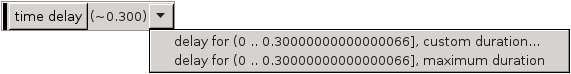
At most 0.30000000000000066 units of time can pass (0.300 in short
form). The first option is to choose a custom duration. The second option is
to choose that maximum duration, similar to clicking the
time delay
button. The following image shows the dialog that is presented to the user to
enter the custom duration:
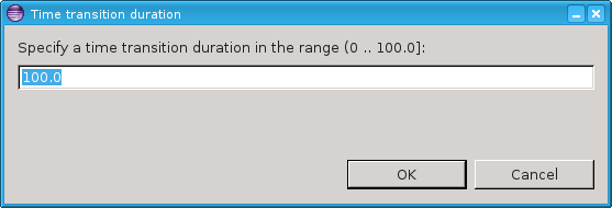
By entering an integer or real number for the duration, that exact amount of time units will pass, after clicking the OK button. If the Cancel button is clicked instead, the choice is canceled, and the user is again free to choose between all available choices.
The reset button makes it possible to reset the simulation to the initial state. The popup menu that can be shown by clicking on the arrow button, has only one option, which the same effect as clicking the button. The following image shows the popup menu:

The undo button makes it possible to undo a single transition, and go back to the state just prior to that transition. The number of transitions that can be undone, is displayed as label between the two buttons.
Clicking the arrow button shows a popup menu with additional options. Menu items are present to undo 1 transition, to undo 2 transitions, to undo 3 transitions, etc, for as many transitions as can be undone. The following image shows an example with two transitions that can be undone:
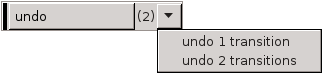
At most 10 such menu items are shown. If more than 10 transitions can be undone, an additional choice is present, that allows entering a custom number of transitions to undo. The following image shows an example with 12 transitions that can be undone:

Selecting that last option will present the user with a dialog, to select the number of transitions to undo:
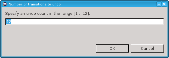
The number of transitions needs to be entered as a positive number, within the given range. Clicking the OK button will undo the requested number of transitions. If the Cancel button is clicked instead, the choice is canceled, and the user is again free to choose between all available choices.
By default, in the interactive GUI input mode, the user is asked to choose, even if for instance there is only one possible transition. Having to choose for every transition can become tiresome. To reduce the number of situations where a choice is required, the semi-automatic mode is available.
Choices that are no longer available due to them being automatically chosen by enabling semi-automatic mode, are not shown in the GUI of the interactive GUI input mode. See also the Availability section above.
By enabling semi-automatic mode to automatically choose time transitions
(option value time), while not automatically choosing the delay durations
of time transitions (option value timedur), time transitions are
automatically chosen, but the user is still asked to choose the duration of the
time transitions. For this choice, all non-time choices are disabled, making
only the time related choices available. The effect of the
time delay
button remains the same, i.e. choosing the maximum
allowed or available delay. The popup menu for the time delay also still shows
the default options, to choose either a specific custom delay duration, or the
maximum duration.
By enabling semi-automatic mode to automatically choose the delay durations of
time transitions (option value timedur), while not automatically choosing
the time transition themselves (option value time), the effect of the
time delay
button changes from choosing the time transition with
the maximum allowed or available delay, to choosing the time transition and
letting the automatic input component
choose the actual delay duration, based on its own configuration. The popup
menu for the time delay then only shows one option, to let the automatic input
component choose, identical to the effect of the
time delay
button.
By closing the GUI of the interactive GUI input component, no more interactive choices can be made. The next time an interactive choice is to be made, simulation terminates.
While an interactive choice is to be made via the GUI, the red stop button of the Eclipse console does not function. Once a choice is made, simulation will terminate.
Automatic input mode
In the automatic input mode, the simulator automatically chooses transitions as well time transition durations. How the simulator chooses however, can be influenced using options. These options are explained below. The final section of this page explains the limitations of using these options.
In the automatic input mode, the simulator automatically chooses the transitions to take, without any user interaction. The choice that is made can however be influenced using the Automatic mode choice algorithm option (Input category). The following choices are available:
-
First transition.
-
Last transition.
-
Random transition (random seed).
-
Random transition (specific seed).
The options to choose the first or last transition do exactly what they state,
i.e. they choose the first respectively the last transition from the list of
possible transitions. Note that event transitions are always listed before
time transitions, but event transitions can only be listed together with time
transitions if environment events are
present. Also note that if transitions for the tau event are present, they
are listed after the transitions for all other events.
The other two options randomly choose a transition from the possible transitions. If a random seed (for the random number generator) is used, each simulation will potentially choose a different trace. In this case, the seed that is used, is printed to the console at the start of the simulation. If a specific seed is used, then the choices are still random, but can be reproduced. Each simulation, using random automatic input mode, with the same seed, for the same specification, should lead to the same trace. Seeds are integer numbers from the range [0 .. 230].
In the automatic input mode, the simulator automatically chooses the durations of the time transitions, without any user interaction. The choice that is made can however be influenced using the Automatic mode time transition duration option (Input category). The following choices are available:
-
Maximum allowed duration.
-
Random duration (random seed).
-
Random duration (specific seed).
The option to choose the maximum allowed duration does exactly what it states, i.e. it chooses the maximum allowed duration for each time transition, until the next potential state event.
The other two options randomly choose a duration for the time transitions. For both options, a uniform random distribution is used, which is sampled to obtain the time at which time transitions are to be 'interrupted' or 'cut off'. The upper bound (exclusive) of the uniform random distribution is to be provided by the user. You can think of these random options as adding an extra automaton to the specification, that could look as follows:
automaton auto_time_trans_duration:
const real UPPER = ...;
disc dist real d = uniform(0.0, UPPER);
disc real timeToWait;
cont t der 1.0;
location sampling:
initial;
edge do (timeToWait, d) := sample d goto waiting;
location waiting:
edge when t >= timeToWait do t := 0.0 goto sampling;
endThe upper bound of the uniform real distribution (UPPER > 0), is provided
by the user. A sample is taken from the distribution, indicating the time to
wait before the time transition is to be interrupted. Once that much time has
elapsed, a new sample is taken, and the process repeats itself. The actual
implementation is slightly different, in that no actual automaton is added,
no additional tau transitions result from using this option, and no zero
length time transitions are chosen. However, the effect is very similar.
So, say the user wants to use a uniform distribution over interval [0 .. 10). The simulator takes a sample, say 3.0. Assume we then get a time transition for at most 0.5 time units. We take that entire transition and are left with 2.5 remaining time units (3.0 - 0.5). If we then get another time transition for at most 1.2 time units, we take that one entirely as well. We are left with 1.3 (2.5 - 1.2) time units. If we would then get a time transition for at most 5.0 time units, the automatic input component ensures that we instead get a time transition for at most 1.3 time units, instead of one for at most 5.0 time units. Since we choose to interrupt after 1.3 time units anyway, there is no reason to compute the remainder of the time transition after those 1.3 time units. We choose the entire time transition of 1.3 time units, and compute a new sample. The simulator then once again calculates new transitions, and the process repeats. The next time transition that is calculated will be for the remaining 3.7 (5.0 - 1.3) time units, unless it is interrupted again before that time, i.e. if the new sample is smaller than 3.7.
If a random seed (for the random number generator) is used, each simulation will potentially choose a different trace. In this case, the seed that is used, is printed to the console at the start of the simulation. If a specific seed is used, then the choices are still random, but can be reproduced. Each simulation, using random automatic time transition duration, with the same seed, for the same specification, should lead to the same trace. Seeds are integer numbers from the range [0 .. 230].
The random durations are particularly useful in combination with environment events, as it allows the environment events to be chosen at the time the time transition is interrupted. That is, it allows the environment events to occur at random times. Using this option, the user can specify the distribution used for 'cutting up' the time transitions, and thus the possible moments when environment events can potentially take place. This is in addition to the state events, at which the environment events can also be chosen. These new additional possibilities however, are not influenced by the occurrence rate of the events of the system, and allow more control for the user. In particular for cases where the simulation allows infinite time transitions (no state events), the infinite time transitions can then be interrupted to allow environment events to take place.
Using the two options described above, and choosing random for each of them, introduces a certain degree of randomness to the trace that the simulator will explore. This randomness however, is rather limited. For one, the distributions that are used are mostly fixed, as the options don’t allow using for instance an exponential distribution. Furthermore, there is no way to specify the distribution for events individually, and it is not possible to specify the distribution between event transitions and time transitions. Concretely, the options for instance don’t enforce that environment events get chosen. They may be chosen when the time transitions are interrupted, or at state events, but that is not guaranteed, as the simulator may choose the time transition again, after the interruption.
The options provide a lightweight, quick, and easy to use approach to adding some randomness. If more control is needed, the environment can instead be modeled explicitly in the CIF model, thus defining when the environment events may or will occur. One way to accomplish this, is by adding a use case.
Trace input mode
In the trace input mode, the simulator automatically chooses transitions as well as time transition durations, based on a user provided trace file.
If the trace input mode is used, the
Trace input file
option
(Input
category) can be used to specify the path to the trace file.
If the path is not explicitly specified, the input CIF file path is used, where
the .cif file extension is removed if present, and a .trace file
extension is added.
The trace file uses a line based file format. Leading (at the beginning of the
line) and trailing (at the end of the line) whitespace is ignored. Empty lines
as well as lines starting with a hash character (#) are ignored as well.
Lines starting with a hash character can be used as comment lines. All other
lines contain commands.
There are two types of commands: option commands and non-option commands. The option commands must always be before the non-option commands.
All option commands use the option NAME VALUE syntax, where NAME is the
name of the option, and VALUE is the value of the option. Option commands
must be specified in the trace file, before any other (non-option) commands.
The remainder of this section explains the available options.
-
option strict on/off (default
off)The strict option can be used to specify whether a strict match is expected for an event. If strict mode is on (option strict on), it is considered an error if more than one transition is possible for an event from the trace. If strict mode is off (option strict off), and there are multiple possible transitions for an event from the trace, the automatic input component is asked to choose between those possible transitions for that single event, based on its own configuration. The strict option applies only to events, not time delays.
-
option time off/implicit/explicit (default
implicit)The time option can be used to specify the time mode to use. If the time mode is off (option time off) , time passage is not allowed. That is, time delays/transitions are never chosen, and the value of variable time remains zero during the entire simulation. For this mode, the time command is not allowed.
If the time mode is implicit (option time implicit), time delays are chosen if necessary. The simulator will use the least amount of time passage possible, to still enable the events as specified in the trace. In other words, if an event is possible no time delays occur, and otherwise the simulator delays for as long as is needed until the event becomes enabled. For this mode, the time command is not allowed.
If the time mode is explicit (option time explicit), time delays are only possible if the time command explicitly allows time passage.
The transition commands can be used to specify the actual trace itself, to choose specific transitions. The following commands are available:
-
event NAME
The event command indicates that an event transition should be taken. The event to choose is indicated by the
NAMEpart, which must be an absolute name of an event. For an automatonawith an evente,NAMEmust bea.e, and the full command would thus be eventa.e.If CIF textual syntax keyword are used as names for events (such as
plant), then they must be escaped in.ciffiles (e.g.$plant). For event commands however, no escape characters ($) should be used in event names.If the specified event is not enabled in the current state, the simulator checks whether time passage is allowed and possible. For the off time mode, time passage is not allowed, and the simulation results in deadlock. For the implicit time mode, the simulator delays if a time transition is possible, and otherwise simulation results in deadlock. For the explicit time mode, if the current event command was preceded by an explicit time command, the simulator delays if a time transition is possible, and otherwise (current command not preceded by time command or no time transition possible) simulation results in deadlock. Upon deadlock, simulation ends, and a warning is printed to the console to indicate the event that was not enabled.
If multiple transitions are possible for the event, due to non-determinism, the strict option (see above) determines if and how the simulator proceeds.
-
time
The time command explicitly indicates that time is allowed to pass, i.e. the simulator may delay by choosing a time transition. This command is only allowed for the explicit time mode.
The time command does not ensure that time passes. It specifies that time passage is allowed, not that it is required. Specifying the time command multiple times without an intermediate event command has the same effect as specifying the time command only once. That is, it doesn’t matter how many times you allow time passage, once is enough.
The commands from the trace file are processed in the order they occur in the trace file. After all commands have been used to select transitions, and no more commands are available, the simulation ends. The simulator indicates the simulation has terminated at the request of the user, as the user did not include any more commands in the trace file.
Simulation is also terminated if deadlock occurs or the user-specified simulation end time is reached, even if more (unprocessed) commands are still available.
SVG input mode
In the SVG input mode, the SVG images that are used for SVG visualization can be used to interactively control the simulation. Since the SVG images are reused, using the SVG input mode requires the use of SVG visualization.
The idea is that certain SVG elements are coupled (mapped) to events from the CIF specification. Clicking on those graphical elements then results in the corresponding event being executed by the simulator. This way, the user interface of a system can be modeled graphically, and can be coupled to the specification (during simulation), by means of events. The user interface of the system is thus part of the specification, but is controlled interactively at runtime (during simulation) by the user.
The events that are coupled to visualization elements are called SVG interactive events or SVG input events.
Topics
CIF/SVG input mappings couple ids of SVG elements to events from the CIF specification. CIF/SVG input mappings are CIF/SVG declarations, similar to CIF/SVG output mappings. If the CIF specification contains input mappings, and SVG input mode is not used, the input mappings are simply ignored.
The simplest form of an SVG input mapping maps to a single event. For instance:
svgin id "button" event machine.button.toggle;This input mapping maps the SVG element with
id button to the
machine.button.toggle event from the CIF specification.
Every input mapping must specify the id of an SVG element, and an SVG element with that id must exist in the SVG image. Specifying an input mapping for an SVG element turns that SVG element into an interactive SVG element. Note that groups may be used as interactive SVG elements as well.
if event input mappingSometimes, the simple single event input mapping is not enough. Consider for instance the following CIF specification:
automaton button:
event u_pushed, u_released;
location Released:
initial;
edge u_pushed goto Pushed;
location Pushed:
edge u_released goto Released;
endThis specification models a button that is initially released (location
Released). When the button is pushed (event u_pushed), the location is
updated to Pushed. If we now want to couple a graphical representation of
a button to this CIF specification, the event to choose depends on the current
location of the button automaton. This can be mapped using an
if event input mapping, as follows:
svgin id "button" event
if button.Released: button.u_pushed
elif button.Pushed: button.u_released
end;If the button is released, the u_pushed event is chosen, and if the button
is pushed, the u_released event is chosen.
The if event input mappings are essentially an if expressions that
result in an event rather than a value. The conditions (such as
button.Released are guard expressions that evaluates to a boolean value.
The guard expressions may be arbitrary expressions, similar to the use of
expressions in output mappings.
If a condition holds, the corresponding event is chosen. The entries are
processed in the order they are specified: if the first guard (of the if)
holds, the first event is chosen, otherwise if the second guard
(of an elif) holds, the second event is chosen, etc.
The last part of the if is allowed to be an else, to indicate that
if none of the previous guards hold, the event of the else is to be chosen.
Using an else entry is optional, but if used, there may only be one such
entry, and it must be the last entry of the input mapping.
Similar to output mappings, all input mappings must be unique, per SVG image. That is, no two input mappings for the same SVG image may use the same SVG element id. Note that it is allowed to have an input mapping and an output mapping (or even multiple output mappings) for the same SVG element.
Input mappings must be complete. Single event input mappings are always
complete, as are if event input mappings with an else. For if
event input mappings without an else, at least one of the guards must hold.
If none of the guards holds, the mapping results in a runtime error during
simulation.
This page explains the use of the SVG input mode of the CIF simulator at runtime (during simulation).
During simulation, as long as none of the interactive SVG elements (the SVG elements for which an input mapping exists) are clicked, the corresponding events are never chosen. For the other events (the non-interactive events), a choice is made using the automatic input component. The automatic input component makes a choice based on its own settings.
When moving over one of the interactive SVG elements of the SVG visualization, using the mouse pointer, the border of the SVG element is highlighted in red. This makes it easier to identify the interactive SVG elements in the SVG visualizer. When an interactive SVG element is clicked, the color is changed from red to green, for as long as the mouse button is not released.
The mouse click (and not the release) makes that the input component will interrupt any time transition that is currently being taken by the simulator. Then, when asked to choose a next transition, it will apply the input mapping for the interactive SVG element that was clicked. The event that results from the input mapping is then chosen. If the event is not enabled at that time, simulation ends in deadlock. To prevent such deadlocks, you can use a monitor automaton. If multiple transitions are possible for that event, the choice (between the transitions for that event only) is deferred to the automatic input component, which makes a choice based on its own settings. Note that multiple transitions are only possible if complete mode is enabled.
The SVG input mode allows interactively choosing certain events by clicking on interactive elements of an SVG image. The SVG input mode is however not officially an interactive input mode.
The image plays the part of the environment. Whenever an interactive element is clicked, the element is added to a queue. If a user quickly clicks the same element multiple times, or quickly clicks different elements, they are all stored in the queue, and the queue can grow. The transition to take is automatically chosen, based on the queue of events. If the queue is empty, the environment (the SVG image and the user) doesn’t allow the interactive events. If the queue is not empty, the environment allows exactly one interactive event, the one at the head of the queue. The model, together with the queue, form a closed model, without further interaction. Each interactive SVG element that is clicked, will be used in the order they were clicked, to choose transitions.
The SVG input mode internally acts as an automated input mode, that makes choices about which transitions to take, without further user interaction. Since no further user interaction is possible, undo and reset are also not supported.
The console debugging output for CIF/SVG mappings includes debugging output for SVG input mappings. Input mappings that encounter runtime errors have stack traces similar to those of output mappings.
SVG input is usually combined with real-time simulation. Clicking an interactive SVG element results in the application of an input mapping, which results in an event. That event is put in the queue. If a time transition is being taken by the simulator, the simulator will continue to take that time transition until the input component interrupts it. However, an input component can only interrupt a time transition during intermediate frames. As such, choosing a low frame rate (typically less than 10 frames per second) can significantly reduce the responsiveness of the SVG input.
Hovering interactive SVG elements highlights their borders in red. This too becomes less responsive when a low frame rate is used.
It is possible to make a group of SVG elements (an svg:g element) an
interactive element. By doing so, all the elements that are part of the group
together become one single interactive element.
One practical example where this is very useful, is for buttons with a text label. In SVG, this requires the use of a rectangle and a text label. To ensure that clicking either one of them results in the same event, group the rectangle and text label together in a group. Then assign an id to the group and use that id in an input mapping. During simulation, when hovering over either the rectangle or the text label, both will will be highlighted. Clicking on either of them results in the corresponding input mapping being applied, and the resulting event being chosen by the SVG input component.
In general, if an SVG image is clicked, the simulator will figure out on which graphical element the user clicked. If that element is itself an interactive SVG element, then the corresponding mapping is applied. If it is not an interactive SVG element, its parent (which may be a group) is checked. If the parent is not an interactive SVG element either, the parent of the parent is checked, etc. If none of the ancestors is an interactive SVG element, clicking the element has no effect on the simulation. Because of this behavior, it is strongly recommended not to make a child (or descendant in general) of an interactive SVG element interactive as well.
Semi-automatic mode
By default, in the interactive console and GUI input modes, the user is asked to choose, even if for instance there is only one possible transition. Having to choose for every transition can become tiresome. To reduce the number of situations where input is required, the semi-automatic mode is available. Semi-automatic mode allows the simulator to automatically choose certain transitions, while leaving the remaining choices for the user. The following choices can be automatically made by the simulator, in semi-automatic mode:
-
Automatically choose a transition if there is only one transition possible.
-
Automatically choose time transitions, regardless of how many transitions are possible.
-
Automatically choose the delay duration of time transitions.
-
Automatically choose event transitions (for certain events), regardless of how many transitions are possible.
Each of these possible automatic choices can be individually enabled, through the Interactive mode automatic transition choice option (Input category). As value for the option, comma separated filters should be supplied. The following filters are available:
-
1to automatically choose a transition if there is only one transition possible. -
timeto automatically choose time transitions. -
timedurto automatically choose the delay duration of time transitions. -
The name of an event, to automatically choose event transitions for that event.
-
urgentto automatically choose event transitions for all urgent (non-environment) events.
For events, the absolute names of the events are used. That is, for an
automaton a, with an event e, the absolute name of the event is
a.e. If CIF textual syntax keyword are used as names for events (such as
plant), then they must be escaped in .cif files ($plant). For
filters however, all escape characters ($) in event names are ignored.
The * character can be used as wildcard, to indicate zero or more
characters. The special urgent event filter matches all
urgent events of the specification. If an
event filter doesn’t match any of the events of the CIF model, a warning is
printed to the console. If a filter doesn’t have any effect, because a previous
filter already turned ensured that the matching events into are automatically
chosen, a warning is printed as well.
As an example, option value 1, g*, t* consist of three filters: 1,
g*, and t*. The first filter indicates that the simulator should
automatically choose a transition if there is only one transition possible. The
second and third filters indicate that the simulator should also automatically
choose all events starting with an g or a t, such as g, g1,
go, etc. Note that the wildcards apply only to events, so t* does not
mean that time transitions should be automatically chosen. The t* filter
always matches the tau event, as that event is implicitly always present.
If an automatic choice can be made, given the filter and the possible transitions, the transitions are filtered to only keep the ones that can be chosen automatically, and they are sent to the automatic input component, which then makes the actual choice, depending on its own configuration. Similarly, if the delay duration of a time transition is to be automatically chosen, the automatic input component is asked to choose, based on its own configuration.
State history
The CIF simulator can be used to explore the state space of a CIF model. It is possible to see step by step, what is possible, and choose some transitions. Sometimes, after exploring a bit, you may want to go back a bit, to explore some alternative behavior. Obviously, you can terminate the simulation, and start a new one. There are several downsides to this. First, you have to start from the initial state again, while you may want to only go back a few states, and continue from there. Second, restarting the simulator may take some time, especially for large models. Third, if you use several visualizations, you may have to layout them again, to be able to see all of them.
To make it easier to explore alternatives, the simulator supports resetting the simulation to the initial state, as well as undoing a certain number of transitions. This page explains that functionality in more detail.
The History option (Input category) can be used to enable or disable history. By default history is enabled. Using the option, it can be disabled. Disabling history disables both the reset and the undo functionality, which ensures no time or memory is consumed in keeping track of earlier states.
If history is enabled, it only has an effect if an interactive input mode is used. Other (automatic) input modes will never perform a reset or undo. That is, the simulator will not keep track of any history states, unless an interactive (either fully interactive or semi-automatic) input mode is used, and history is enabled via the History option.
In order for the simulator to be able to go back to earlier states, it will need to remember those states. To that end, the simulator can store states that it has encountered in a state stack. The initial state is remembered separately. So, initially, the following is remembered:

Here, state 0 is the initial state. After two transitions are taken, the
following is remembered:

Here, two more states, numbered 1 and 2 are remembered. After one more
transitions is taken, the following is remembered:

Here, one more state, numbered 3, is remembered. In each case, the last
shown state is the current state. If we undo two transitions, the following is
remembered:

As two transitions are undone, their resulting states (the last two states) are forgotten. If we take one more transition after the undo, we get the following:
This state 2 may be the same one as before, or it may be a new one, if a
different simulation choice was made. If we reset the simulation, we forget all
but the initial state, and end with up:
For long simulations, a lot of states will need to be remembered. Each state that needs to be remembered costs some amount of memory. To limit the amount of states that are remembered, the History size option (Input category) can be used.
If set to infinite, there is no limit to the amount of states that can be
remembered. If set to a finite (non-negative) number, at most the given number
of states are remembered, apart from the initial state. So, if set to zero,
only the initial state is remembered. If set to one, one additional state is
remembered, etc. The default history size is 100 states. Since if set to
zero, only the initial state is remembered, this completely disables undo
functionality.
By introducing a maximum number of states that can be remembered, this also
introduces a maximum number of transitions that can be undone. Let’s consider a
history size of 3. After three transitions, the following is remembered:
State 3 is the current state. It is possible to undo one, two, or three
transitions, going back to states 2, 1, and 0, respectively. Now
consider what happens when we take another transition. We already remember
three states besides the initial state, and have thus reached the maximum
number of states to remember. By remembering the new target state of the fourth
transition, we need to let go of state 1, as it is the oldest remembered
state, not taking into account the initial state. After this fourth transition,
the following is remembered:

State 4 is the current state. We can undo one transition, to go back to
state 3. We can also undo two transitions, to go back to state 2.
However, as we forgot all about state 1, we can’t undo three transitions.
Due to the gap between states 0 and 2, we can’t undo past state
2. As you can see from this example, for a history size of 3, we can undo
at most 3 transitions when there is no gap, and at most 2 transitions when
there is a gap.
If history is disabled, reset is not available. If history is enabled, reset is available only if the current state is not the initial state. That is, reset is enabled for every state, except for the initial state.
If history is disabled, or the history size is zero, undo is not available. If
history is enabled, and the history size is positive or infinite, undo is
available. The number of transitions that can be undone depends on the number
of states that is remembered. If n states are currently remembered,
excluding the initial state, then n - 1 transitions can be undone, at the
least. If there is no gap, and the current state is not the initial state, then
n transitions can be undone.
Reset and undo are only supported by interactive input modes, as explained above.
When the simulator interactively asks the user to choose between some possible transitions, it may also provide the possibility to reset the simulation to the initial state, or to undo some transitions. The details on how the different choices are presented, and how the choice can be made, are explained in the documentation for each of the interactive input modes.
If no transitions are possible, for instance due to deadlock or reaching the end-user provided simulation end time, the simulator may interactively ask the user to choose between termination of the simulation, resetting the simulation to the initial state, or undoing some transitions. This choice is only presented if either reset or undo is enabled, as otherwise there is no choice to make. The details on how the different choices are presented, and how the choice can be made, are explained in the documentation for each of the interactive input modes.
By using semi-automatic mode, a purely interactive input mode, can be made semi-automatic. This can lead to unexpected results, in combination with reset and undo.
Consider a situation where four transitions have been taken. The first transition was manually chosen, as was the third. The second and fourth transition were automatically chosen. The user is asked to interactively choose the fifth transition. Consider what happens if the user chooses to undo three transitions. The simulator goes back to the state reached after the first transition. The possible transitions are the same as the first time they were calculated. An automatic choice was made for the second transition, so one will also be made the second time around. So, after the second transition is once again automatically chosen, the user is interactively asked to choose the third transition. So, instead of undoing three transitions and getting a choice for the second transition, three transitions are undone, a second transition is automatically chosen, and the user is asked to choose for the third transition.
Similarly, undoing the fourth transition, will result in a fourth transition being automatically chosen again. If the same choice is made as before, undoing the fourth transition has no effect.
Resetting the simulation to the initial state, will not lead to the user being able to choose the transition to take from the initial state, if the first transition is automatically chosen.
Environment events
By default, the CIF simulator treats all events are urgent. That is, whenever a transition is possible for any event, time may not progress. In other words, events take priority over time passage. However, not all events should be urgent. As such, the simulator has an Environment events option (Input category), that makes it possible to let the simulator know about the environment events (non-urgent events). An example of an environment event (non-urgent event) is a button that can be pushed. The button can always be pushed, now or in the future. The corresponding event is thus always enabled, but time should still be able to progress, as the event may not actually happen at this time.
As value for the
Environment events
option, comma separated
filters should be supplied. Each filter specifies one or more environment
events. The absolute names of the events are used. That is, for an automaton
a, with an event e, the absolute name of the event is a.e. If CIF
textual syntax keyword are used as names for events (such as plant),
then they must be escaped in .cif files ($plant). For filters however,
all escape characters ($) in event names are ignored. The * character
can be used as wildcard, to indicate zero or more characters. The special
svg filter can be used to turn all
SVG interactive/input events into
environment (non-urgent) events. If a filter doesn’t match any of the events of
the CIF model, a warning is printed to the console. If a filter doesn’t have
any effect, because a previous filter already turned the matching events into
environment events, a warning is printed as well.
As an example, option value e, a.e, f*, t* consists of four filters: e,
a.e, f*, and t*. The first filter indicates that event e is an
environment event. The second filter indicates that event e in automaton
a is an environment event. The third filter indicates that all events
whose absolute name starts with an f are environment events. This could
include events f, f1, foo, f.e, etc. The fourth filter is
similar to the third filter, but uses character t as a prefix, rather than
character f. The t* filter always matches the tau event, as that
event is implicitly always present.
Input modes
By default, the simulator does not know which events of the model are environment events (non-urgent events). By letting the simulator know about them, it can properly simulate them with non-urgent semantics. The CIF simulator however, has several input modes. This section discusses for each input mode, the influence of environment events, and their practical use.
-
Interactive console input mode
When using the interactive console input mode, the simulator will interactively ask the user to choose transitions, from the list of possible transitions printed to the console.
If however the CIF model contains events that are always enabled (such as a button that can always be pushed), time may never progress. The simulator treats all events as urgent. By specifying the always enabled events as environment events, those events become non-urgent, and the user is free to choose between those environment events and time passage (time transitions). If combined with the semi-automatic mode for the urgent events, the user can choose the environment events and time transitions, while the other/urgent events are automatically chosen by the simulator, reducing the number of choices the user has to make.
-
When using the interactive GUI input mode, the simulator will interactively ask the user to choose transitions, using a GUI (Graphical User Interface).
If however the CIF model contains events that are always enabled (such as a button that can always be pushed), time may never progress. The simulator treats all events as urgent. By specifying the always enabled events as environment events, those events become non-urgent, and the user is free to choose between those environment events and time passage (time transitions). If combined with the semi-automatic mode for the urgent events, the user can choose the environment events and time transitions, while the other/urgent events are automatically chosen by the simulator, reducing the number of choices the user has to make.
-
When using the automatic input mode, the simulator will automatically choose transitions, based on certain criteria. If the CIF model contains a use case, the simulator automatically simulates that use case.
If however the CIF model contains events that are always enabled (such as a button that can always be pushed), time may never progress. The simulator treats all events as urgent. By specifying the always enabled events as environment events, those events become non-urgent, and the simulator is free to choose between those environment events and time passage (time transitions). If combined with the random automatic mode choice algorithm, and random automatic mode time transition duration, this allows for the automatic validation of arbitrary traces.
-
When using the SVG input mode, the simulator will automatically choose transitions, based on certain criteria. The environment events are usually coupled to the SVG image (using CIF/SVG input mappings). This ensures that the environment events are only enabled when the corresponding interactive element of the image is clicked by the user. The SVG image plays the role of the environment, closing the system. If the SVG image only partially closes the system, the remaining environment events can be specified, similar to the way they are specified for the automatic input mode.
Supervisory control application domain
This section discusses environment events in the application domain of supervisory control, where the system consists of a plant (the hardware), and a supervisor (or other controller that restricts the plant behavior).
Informally, we can distinguish the following types of events:
-
Controller events
Controller events are those events that are initiated by a controller, such as a supervisor. These events are usually controllable events. However, if supervisor synthesis is not used, the events need not necessarily be controllable.
For controller events, the behavior is usually fully specified in the CIF model. That is, if the CIF model contains both the plant and the controller, the CIF model determines when the events are enabled, and when they are disabled. The controller events should happen as soon as they are enabled. That is, once the controller determines that for instance a motor should be turned on, the motor should be turned on without further delays. Thus, controller events are urgent.
For low-level controllers, the events generally correspond directly to the events of the actuators. For instance, a controller may turn a lamp on or off. For higher level controllers however, there usually is no such direct relation. Furthermore, internal events of the controller (usually event
tau, or other events that are neither controllable nor uncontrollable), are considered controller events as well. -
Plant events
Plant events are those events that are initiated by the plants. These events are usually uncontrollable events. However, if supervisor synthesis is not used, the events need not necessarily be uncontrollable.
For plant events, the behavior is usually fully specified in the CIF model. The CIF model models exactly when the events become enabled. For instance, when an elevator moves and reaches its top position, the event that indicates that 'the top position sensor goes on' becomes enabled, and should be executed at that time. That is, the plant model models/follows the physical behavior, and determines when the plants events are enabled. This behavior is fully specified and known, and further delays are undesirable. As such, plant events are urgent.
For low-level plants, the events generally correspond directly to the events of sensors. Typical examples include limit sensors, such as the elevator top position sensor described above, and sensors that detect products throughout the system. For higher level plants however, there usually is no such direct relation. Furthermore, internal events of the plants (usually event
tau, or other events that are neither controllable nor uncontrollable), may be considered plant events as well. -
Environment events
Environment events are those events that are initiated by the environment (anything outside and the plants and the controller). These events are usually uncontrollable events. However, if supervisor synthesis is not used, the events need not necessarily be uncontrollable.
The CIF model only observes or monitors the environment events. The environment (outside of the behavior specified in the CIF model), determines when, if ever, the events actually happen, and thus defines their behavior. From the point of view of the CIF model, the environment events can happen at any time, and as such the CIF model allows them at all times. The behavior is left completely unrestricted/free in the CIF specification, as it is unknown when the events will actually happen. Since time may pass before these events actually happen (as determined by the environment, rather than the CIF model), these events are thus non-urgent (from the point of view of the CIF model). If the CIF model would instead consider them to be urgent, the model would always forbid time to progress, even if the environment does not currently allow any environment event to occur, leading to deadlock.
For low-level plants, the events generally correspond directly to the events of sensors. For instance, the buttons of a user interface can be pushed and released. Other typical examples of environment events include events for other user interface elements, and events that indicate that a product has entered the system, from the environment of the system. For higher level plants however, there usually is no such direct relation. Furthermore, internal events of the plants (usually event
tau, or other events that are neither controllable nor uncontrollable), may be considered plant events as well.
Thus, for plant events as well as for controller events, the CIF model specifies/defines when the events may/should occur, while for environment events the specification always allows them, and lets the environment choose/determine when they actually occur. In other words, plant/controller events originate from within the specification (internal behavior), while environment events originate outside of the specification (external behavior).
A closed system is a system for which the entire behavior is specified in the CIF model. Closed systems have no environment events.
An open system does not model the environment. As such, open systems typically have plant events, controller events, and environment events. The environment events are then unrestricted in the CIF model, leaving the environment (which is not specified) free to determine its own behavior, and thus the behavior (enabledness) of the environment events.
An open system can be closed by adding a use case, which models one possible sequence of behavior of the environment, over time. That is, the added use case eliminates environment events, by defining when they are enabled. Open systems can also be closed by the simulator, as described above for the different input modes.
As an example, consider the following open system:
plant automaton Button:
uncontrollable u_pushed, u_released;
location Released:
initial;
edge u_pushed goto Pushed;
location Pushed:
edge u_released goto Released;
end
plant automaton Lamp:
controllable c_on, c_off;
location Off:
initial;
edge c_on goto On;
location On:
edge c_off goto Off;
end
supervisor automaton ButtonLampController:
location:
initial;
edge Lamp.c_on when Button.Pushed;
edge Lamp.c_off when Button.Released;
endHere we have a simple button and a lamp. The lamp can only be turned on while the button is pushed, and will be turned off as soon as the button is released. The button events are environment events, since it always possible to either push the button, or release it.
By specifying the button events as environment events, and specifying the the lamp events as semi-automatic events, we can use the interactive console input mode or the interactive GUI input mode to try different traces, where we only have to choose between the button events and how much time we want to let pass.
Alternatively, we could add a use case, modeling one possible behavior of a user:
plant automaton User:
cont t der 1.0;
location:
initial;
edge Button.u_pushed, Button.u_released when t >= 1 do t := 0.0;
endThis specifies that the user either pushes or releases the button, after one
unit of time has passed (typically one second). Since clock t is reset each
time, the user repeats this behavior. Thus, the button is pushed after one
second, for one second, after three seconds, for one second, after five
seconds, for one second, etc. This extended model (with use case), can be
simulated using the automatic input mode, as the
User plant automaton closes the system.
Simulation output
The CIF simulator can produce various forms of output.
Console output
The default form of output is to the console. The type of console output to produce, is determined by the Output mode option (General category). The following modes are available:
-
Error: produces only error output. It is recommended not to use this mode. Use the warning mode instead, if you wish to limit the amount of console output.
-
Warning: produces error and warning output. Use this mode to be informed about potential problems, while keeping the amount of console output to a minimum.
-
Normal: produces error, warning, and normal output. This is the default output mode. The information that is printed to the console for normal output can be configured using the Normal output option.
-
Debug: produces error, warning, normal, and debug output. This mode can be used to print additional debugging information to the console. The information that is printed to the console for normal output can be configured using the Debug output option.
The simulator can thus produce two types of configurable console output:
Output components
Besides console output, the simulator also features a powerful and extensible output framework. This framework allows for the addition of output components, such as visualizers. The following output components are currently available:
Other topics
Normal console output
Normal console output mainly focuses on the state of the specification, and the progress of the simulation.
The following types of normal output are available:
-
The initial state [
state-init] (default)Prints the initial state to the console.
-
The target states [
state-target] (default)Prints all target states to the console. This includes all states reached by event transitions and time transitions. Specifically, it excludes the initial state, and it includes the final/deadlock state.
-
The final state [
state-final]Prints the final state to the console, regardless of whether or not the final state is a deadlock state.
-
The deadlock state [
state-deadlock]Prints the final state to the console, but only if it is a deadlock state.
-
The intermediate states [
state-intermediate]Prints all intermediate states to the console. Intermediate states are the states that are used to generate intermediate frames, for smooth visualizations. The intermediate states are generated for states between the start and end states of time transitions, when real-time simulation is enabled. Note that this does not include the initial state, target states, and final/deadlock states.
-
The algebraic variables as part of the state [
state-alg-vars] (default)Prints the algebraic variables (derived state) as part of the state. This applies to all states, including the states for intermediate frames. If no state information is printed, this output type has no effect. Disabling printing of algebraic variables excludes algebraic variables, regardless of whether state filtering includes or excludes them.
-
The derivatives as part of the state [
state-derivs] (default)Prints the derivatives of the continuous variables (derived state) as part of the state. This applies to all states, including the states for intermediate frames. If no state information is printed, this output type has no effect. The derivative of variable
timeis not included. Disabling printing of derivatives excludes derivatives, regardless of whether state filtering includes or excludes them. -
The possible transitions (for interactive console choice only) [
trans-minimal]Prints the possible transitions to the console, if the interactive console input mode is used. Multiple possible transition are always printed. Single possible transitions are only printed if automatic choice for a single possible transition is disabled. Nothing is printed if no transitions are possible.
-
The possible transitions (for interactive console choice, or if more than one transition) [
trans-default]Similar to 'interactive console choice only', but additionally always prints the possible transitions, if there are multiple possible transitions, regardless of the input mode.
-
The possible transitions (always) [
trans-always]Always print the possible transitions to the console, regardless of the input mode, and the number of possible transitions. However, nothing is printed if no transitions are possible.
-
The chosen transitions [
chosen-trans] (default)Prints the chosen transitions (the transitions that are about to be taken), to the console.
-
The interrupted transitions [
interrupted-trans] (default)Prints information about interrupted transitions (time transitions that are stopped prematurely) to the console.
-
The simulation result [
sim-rslt] (default)Prints the simulation result the console, at the end of the simulation, if simulation did not result in a runtime error.
-
The random seeds used for the random generators [
seeds] (default)Prints the seeds used for the random generators to the console, to allow reproducing the simulation trace. Only if a random seed is used, is the seed printed. That is, for user-specified seeds, the seed is not printed. The following seeds may be printed:
-
The seed used for the random automatic mode choice algorithm.
-
The seed used for the random automatic mode time transition duration.
-
The seed used for the first random generator for a stochastic distribution. The seed is only printed if it is used to create a random number generator for at least one stochastic distribution.
-
-
The print declarations output [
print] (default)Prints the output generated by print declarations.
In the option dialog, each of the different types of output can be enabled and disabled individually (Normal output option, Output category).
From the command line, using the -o or --output option, the names of
the different types of normal output, as specified between square brackets,
should be used, separated by commas. The output types indicated with
'(default)' are enabled when default settings are used, i.e. when the
-o or --output option is not used. As an example, consider
-o print,seeds or --output=print,seeds. Only output generated by print
declarations (due to print) and output about the used seeds for random
generators (due to seeds) is enabled, while all other output is disabled.
The output types that are specified using the option replace the default output
types. However, it is also possible to specify additions and removals relative
to the default output, by prefixing output types with a + or -
respectively. For instance, when using -o -print,+trans-always or
--output=-print,+trans-always the default output is used, with print
declarations output excluded from it (due to -print), and with always
printing possible transitions enabled (due to +trans-always). Replacements
(no prefix) may not be combined with additions/removals (+ or -
prefix).
Specifying a replacement output type twice leads to a warning being printed to the console. Adding an output type that is already present or removing an output type that is not present, also leads to a warning being printed.
When printing states, variable time is always printed first. It is followed
by the current location of each of the automata, the current values of the
state variables (the discrete and continuous variables), the current values of
the derivatives of the continuous variables, and the current values of the
algebraic variables. Except for variable time, the state objects are sorted
alphabetically based on their absolute names. For automata with a single
nameless location, the current location is always *.
For variables with a function type and implicit default values, the
default values may include defaultValueFunc, defaultValueFunc2, etc.
When printing the possible transitions, the event transitions are printed
first, followed by the tau transitions, and the time transition. The event
transitions are sorted alphabetically on the names of the events.
By default, when printing states, all state objects are included. Using the Normal output state filters option (Output category), the state objects can be filtered. The Normal output state filters option only has effect if states are printed at all.
As value for the option, comma separated filters should be supplied. Each
filter specifies one or more state objects. The absolute names of the objects
are used. That is, for an automaton a, with a variable x, the absolute
name of the variable object is a.x. If CIF textual syntax keyword are
used as names for events (such as plant), then they must be escaped in
.cif files ($plant). For filters however, all escape characters ($)
in the names are ignored. The * character can be used as wildcard, to
indicate zero or more characters. If a filter doesn’t match any of the state
objects of the CIF model, a warning is printed to the console.
By default, filters include matching state objects. Filters may however be
preceded by a - character, turning them into exclusion filters, which
exclude matching states objects rather than including them. Filters are
processed in the order they are specified, allowing for alternating additions
and removals. If a filter does not result in the addition/removal of any state
objects to/from the filter result, a warning is printed to the console. A
warning is also printed if the entire state is filtered out.
As an example, option value a.*,-a.b*,a.bc* consists of three filters:
a.*, -a.b*, and a.bc*. The first filter indicates that state
objects whose absolute names start with a. are to be included. The second
filter indicates that from those matching state objects, the state objects
whose absolute names start with a.b* are to be excluded. To that result,
the third filter adds those state objects whose absolute names start with
a.bc*. For instance, if a specification contains state objects time,
a.a, a.b a.bb, a.bc, a.b.c, a.bc, a.bcc, and
a.bcd, the result of the three filters is that the following state objects
are displayed: a.a, a.bc, a.bc, a.bcc, and a.bcd.
The default option value (filter) is *.
Regardless of whether the filtered result includes them or not, all algebraic variables and derivatives of continuous variables may be excluded, using the Normal output option.
If profiling is enabled, all normal output is automatically disabled. That is, profiling suppresses all normal output.
Debug console output
The following types of debug output are available:
-
Debug the CIF/SVG declarations [
svg]Prints debugging information to the console, for the CIF/SVG declarations. For more information on this kind of debugging output, see the page on console debugging for CIF/SVG declarations.
-
Debug the parser [
parser]Prints debugging information to the console, for the parser. This information is primarily intended for the developers of the simulator, and not for end users.
-
Debug the generated code (by writing it to disk) [
gen-code]The simulator generates highly optimized code for the specification. Enabling this debugging output, writes the generated code to disk, for further debugging. This information is primarily intended for the developers of the simulator, and not for end users.
-
Debug the ODE solver [
ode]Prints debugging information to the console, for the ODE solver. This information can for instance be used to figure out why a state event (guard change) was missed.
In the option dialog, each of the different types of output can be enabled and disabled individually (Debug output option, Output category).
From the command line, using the -d or --debug option, the names of
the different types of debug output, as specified between square brackets,
should be used, separated by commas. By default, i.e. when not using the
-d or --debug option, all debug output is disabled. As an example,
consider -d parser,svg or --debug=parser,svg. Debug output is printed
for the parser (due to parser) and CIF/SVG declarations (due to svg).
Specifying an output type twice leads to a warning being printed to the console.
Enabling any debug output, automatically changes the output mode to 'debug mode'.
If profiling is enabled, all debug output is automatically disabled. That is, profiling suppresses all debug output.
Print output
The CIF simulator supports several forms of output. By default, simulation results, such as the current state, are printed to the console. While this provides useful information, it can also be useful to generate custom output, tailored to ones specific needs. To allow this, the CIF simulator supports print output.
Simulation using the CIF simulator results in a trace. A trace consists of the states that are encountered and the transitions that are taken, during the simulation. The print output declarations allow specifying for which transitions text should be printed (for instance only for transitions for a certain event), when the text should be printed (for instance before or after the transition), where the text should be printed (for instance to a file), and what text should be printed.
Print output declarations are an extension to the CIF language, and can be specified directly in the CIF specification. They are only used to couple the model to textual output. They don’t influence the behavior of the model itself. The CIF text editor provides full integration for the print output declarations extension, complete with syntax highlighting, background validation, etc.
Print output can be used to generate text that after simulation is further processed, for instance for visualization or for analysis using statistical software. Print output can also be useful for debugging,
This example serves only to give a quick taste of what print output declarations look like:
printfile "out.txt";
print x for e;This example prints the value of variable x to a file out.txt each
time after a transition for event e is taken.
The tutorials introduce print declarations and text formatting, they explain the general idea behind them, and they show how to use them, all by means of examples. The tutorials are focused on practical use, and do not cover all uses and other details.
The reference documentation discusses all details related to text output and text formatting. It is much more technical than the tutorials.
This tutorial explains print output by means of examples. It does not explain all uses of print output, and all details related to print output. For those details, see the reference documentation instead.
In this tutorial, when printed console output is shown, all output that the simulator can generate other than output for print declarations, is omitted.
Before we start with the examples, the Example model and simulation trace section introduces the example model and simulation trace on which the examples are based. Then, the following examples are explained in detail:
The examples of print output in this tutorial all make use of the same CIF model:
automaton buffer:
event add, remove;
disc int cnt = 5;
location:
initial;
edge add when cnt < 10 do cnt := cnt + 1;
edge remove when cnt > 0 do cnt := cnt - 1;
endThe buffer initially contains five items (cnt = 5). As long as there
is room in the buffer (cnt < 10), an item can be added (event add) to
the buffer. As long as the buffer is not empty (cnt > 0), an item can be
removed (event remove) from the buffer. During simulation, it is possible
to choose between adding an item to the
buffer, and removing an item from the buffer. The following is a potential
simulation trace:

In the initial state (S1), variable cnt has value 5. An item is then
added (transition for the event add), resulting in a new state (S2), where
cnt has value 6. After that, another item is added, leading to state
S3, where cnt has value 7. Finally, an item is removed by means of a
transition for event remove, leading to state S4, where cnt has value
6 again.
If we want to print for every state (S1 through S4), the number of items in the
buffer, we could add the following print declaration to automaton buffer:
print cnt;Then, as a result of this print declaration, the following text is printed to the console:
5
6
7
6That is, for every state (S1 through S4), the value of variable cnt is
printed, on a new line.
Consider the following print declarations:
print cnt file "a.txt";
print cnt * 2 file "b.txt";The first print declaration results in the number of items in the buffer being
printed for every state of the simulation trace, to a file named a.txt. The
second print declaration prints the number of items in the buffer multiplied by
two, to a file named b.txt. These declarations use local file declarations
to specify the file to which output is to be written. It is also possible to
use global print file declarations:
printfile "ab.txt";
print cnt;
print cnt * 2;The print file declaration declares that output of this scope is to be printed
to a file named ab.txt. The two print declarations don’t specify a local
file declaration, and thus use the default file for their scope, in this case
file ab.txt. Alternating lines with the number of items in the buffer and
twice that amount are thus printed to that file.
If we want to print for every state, whether the buffer contains an odd or even
number of items, we could add the following print declaration to automaton
buffer:
print if cnt mod 2 = 0: "even" else "odd" end;Then, as a result of this print declaration, the following text is printed to the console:
odd
even
odd
evenIf we want to print the number of items in the buffer, but only for states
where the number of items is odd, we could add the following print declaration
to automaton buffer:
print cnt when cnt mod 2 = 1;Then, as a result of this print declaration, the following text is printed to the console:
5
7If we want to print the result of adding an item, that is the new buffer count
after a transition for the add event, we could add the following print
declaration to automaton buffer:
print cnt for add;Then, as a result of this print declaration, the following text is printed to the console:
6
7Since an item is added to the buffer twice, two lines of text are printed.
If we want to print the resulting buffer count after every change to the buffer
(addition or removal), we could add the following print declaration to
automaton buffer:
print cnt for add, remove;Then, as a result of this print declaration, the following text is printed to the console:
6
7
6Two items are added to the buffer, and one item is removed from the buffer, leading to three lines of text being printed.
Since the add and remove events are the only events in the system, and
no edges exist without an event (which would implicitly use the tau event),
the print declaration can also be specified as follows:
print cnt for event;That is, the value of variable cnt is printed after each event transition.
If we want to print the buffer count before and after removal of an item from
the buffer, we could add the following print declaration to automaton
buffer:
print pre cnt post cnt for remove;As a result of this print declaration, the following text is printed to the console:
7
6As only one item is removed for our example trace, two lines of text are
printed, one with the buffer count before the removal (due to pre cnt),
and one with the buffer count after the removal (due to post cnt).
If we want to print for every state (S1 through S4), the number of items in the
buffer, we could add the following print declaration to automaton buffer:
print cnt;If we want to print some text before this, as a header, and some text after
this, as a footer, we could add the following print declaration to the top
level scope of the specification, or to automaton buffer:
print "header" for initial;
print "footer" for final;As a result of the original print declaration, and these two new print declarations, the following text is printed to the console:
header
5
6
7
6
footerIn the example simulation trace given at the top of this page, no passage of time is included. If however a trace includes time passage, it is possible to filter printing to only time transitions. For instance, if we want to print the new time after time passes, we could use the following print declaration:
print time for time;This prints the value of variable time, every time after a time transition.
The first time in the print declaration denotes that the value of variable
time should be printed, and the second time denotes that it should be
printed only after passage of time (after time transitions). As an example,
the following could be printed to the console:
0.005
0.75
3.1
7.9In the ninth example, we
printed the new time value after each time transition. However, initially time
is zero. Since the initial state is not reached via a time transition, time
zero is not printed. We could adapt the print declaration to the following, to
print all unique values of variable time, for all states of the simulation
trace:
print time for initial, time;This initially prints the value of variable time, and also prints it after
every time transition. As an example, the following could be printed to the
console:
0.0
0.005
0.75
3.1
7.9In the example model given at the top of this page, automaton buffer has
only one location. If however an automaton has multiple locations, it may be
useful to print the effect of transitions ending in a certain location, or the
state of the system for transitions starting in a certain location. Consider
the following print declaration:
print x for event when aut.loc;This prints the value of variable x after event transitions leading to a
state where location loc is the current location of automaton aut.
That is, whenever an event transition leads to entering that location, the
value of variable x after that transition is printed. Since self loops have
the same source and target location, this includes self loops. To exclude self
loops, use the following print declaration:
print x for event when pre not aut.loc post aut.loc;This print declaration prints the same text, but only prints it after event
transitions from a state where location loc is not the current location
of automaton aut to a state where location loc is the current location
of automaton aut.
So far in this example, we printed text for transitions ending in a location. To print text for transitions starting in a location, consider the following print declaration:
print pre y for event when pre aut.loc post not aut.loc;This print declaration prints the value of variable y in the state that is
exited by the transition, for all event transitions that start in location
loc of automaton aut, but do end in that same location.
This tutorial explains text formatting by means of examples. It does not explain all uses of text formatting, and all details related to text formatting. For those details, see the Text formatting details page instead.
In this tutorial, when printed console output is shown, all output that the simulator can generate other than output for print declarations, is omitted.
Consider the following CIF specification:
print "Time=" + <string>time;When simulated, it could give the following output:
Time=0.0
Time=3.333333333333336
Time=5.000000000000001
Time=10.0As you can see, due to rounding and simulation imprecision, the length of the
textual representations of the values of time can vary wildly during
simulation. Furthermore, the explicit casts (conversions) from real to string
(<string>) and string concatenation (the + operator) can quickly
become cluttered, and hard to read.
To improve readability of the print declaration, we could adapt the CIF specification to the following:
print fmt("Time=%s", time);Here, manual text construction has been replaced by the use of the fmt
standard library function. The first argument is a format pattern, and the
remaining arguments are the values that are to be included in the text, in
this case the value of variable time. The fmt function ensures that we
no longer have to use casts. We also no longer have to create pieces of text
and concatenate them (using the + operator).
This is a typical use of a format pattern. The print declaration prints the
value that results from text formatting. The value that is used is the value of
variable time. The value of this variable is not used 'as is', but is
instead converted to a textual representation using the format pattern. This
format pattern specifies that the resulting text should start with Time=.
It also specifies that the value (of variable time) should be included at
the end of the textual representation. The %s part of the format pattern is
a format specifier. The %s specifier is the generic specifier that can
convert any type of value to a textual representation.
When simulated, this new specification gives the exact same output as the previous version.
As we saw in the previous section, due to rounding and simulation imprecision,
the length of the generic textual representations of the values of variable
time can vary wildly during simulation. This reduces readability of the
results, as a lot of irrelevant digits are included. Consider the following
alternative CIF specification:
print fmt("Time=%.2f", time);Here, instead of a %s specifier, a %f specifier is used. This specifier
can only be used for real numbers, and indicates that the number should be
formatted as a floating point number in decimal representation. The .2 part
specifies the precision, and indicates that the floating point number in
decimal notation should have exactly two digits after the decimal point. When
simulated, this could give the following output:
Time=0.00
Time=3.33
Time=5.00
Time=10.00In the examples above, we included a single value in the output. Now consider the following CIF specification:
print fmt("%.2f %.2f %.2f", x, y, z);Here, the values of variables x, y, and z are included in the
formatted result. The format pattern includes each of the values (the first
%.2f includes the value of variable x, the second %.2f includes the
value of variable y, etc). The format pattern includes spaces between the
format specifiers (between the %.2f parts), and thus the formatted values
include spaces between them as well. When simulated, this could give the
following output:
1.50 0.00 -3.57
2.34 3.75 5.78
4.71 12345.34 -3.12
-3.25 1.25 99.20Due to some larger values being mixed with shorter values, as well as due to having both positive and negative values, the output is not so easy to read. This can be solved by using the following CIF specification instead:
print fmt("%10.2f %10.2f %10.2f", x, y, z);By including a width of 10, the text is now nicely formatted into columns
of ten characters wide:
---------- ---------- ----------
1.50 0.00 -3.57
2.34 3.75 5.78
4.71 12345.34 -3.12
-3.25 1.25 99.20The first line is not actual output, but is included to make it easier to see
the columns. Not only is the output now nicely put in columns, but due to the
exactly two digits after the dot (.), the dots are now also nicely aligned.
Consider the following CIF specification:
print fmt("%.2f", time);When simulated, this could give the following output:
0.00
1.34
5000.23
2147185402.17As the values of variable time get larger and larger, their textual
representations become longer and longer, and it becomes more and more
difficult to see exactly how large the values are. The following alternative
CIF specification solves this problem:
print fmt("%,.2f", time);The addition of the comma (,) flag ensures that we get the following
output instead:
0.00
1.34
5,000.23
2,147,185,402.17That is, a comma is used in the result as thousand separator, making it
easier to see that the value of variable time is just over two billion,
rather than for instance just over 200 million.
Earlier, we put values in columns. By default, if a width is used, text is right-justified (aligned to the right). We can also justify it to the left, as in this CIF specification:
print fmt("%-10.2d %-10.2d %-10.2d", g, h, i);Here the %d specifier is used instead of the %f specifier. The %d
specifier can only be used for integer values, while the %f specifier can
only be used for real values. Besides a different specifier, the minus (-)
flag is added, and different variables are used as values. After the changes,
the CIF specification could result in the following output:
---------- ---------- ----------
184 3675 2
19350 29 -2956
-17 -964563 235
2946 567 -25072563Once again, the first line is not actual output, but is included to make it
easier to see the columns. Observe how the addition of the - flag resulted
in the right-justified output being changed to left-justified (aligned to the
left) output. The presence of negative numbers makes that the left-most digits
of the columns are not nicely aligned. The following CIF specification solves
this:
print fmt("%-+10.2d %-+10.2d %-+10.2d", x, y, z);The addition of the plus (+) flag means that for non-negative numbers, a
plus (+) character is always included:
---------- ---------- ----------
+184 +3675 +2
+19350 +29 -2956
-17 -964563 +235
+2946 +567 -25072563If preferred, a space can be used instead of a plus, resulting in the following CIF specification:
print fmt("%- 10.2d %- 10.2d %- 10.2d", x, y, z);and the following output:
---------- ---------- ----------
184 3675 2
19350 29 -2956
-17 -964563 235
2946 567 -25072563In this short tutorial, we’ve seen a few forms of text formatting using the
fmt function. However, CIF supports various other specifiers, besides the
%s, %f, and %d specifiers that were used in this tutorial. All
those specifiers support various flags, widths, and precisions, and allow them
to be combined in various ways. For the complete details of text formatting,
see the Text formatting details page.
The core concept of print output is the print declaration. The print declarations allow specifying what to print. They also optionally allow specifying when to print it, how to print it, and to where to print it.
Unlike many programming languages that have print statements, CIF has print declarations. Print declarations are declarative, rather than imperative. Print declarations center on transitions. The following is a schematic overview of a transition:
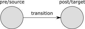
The transition is graphically depicted as an arrow, with a label. The label
denotes the event that occurred, or time for time transitions. Every
transition has a pre or source state,
and a post or target state. The states are graphically depicted as circles,
with a name above them. These names are only used so that they can be referred
to from the text.
The figure thus contains the transition and its immediate environment (its source and target states). Print declarations allow specifying what, how, and when to print, for transitions. Since the transition is the central part, we call this the transition centric view.
Simulation using the CIF simulator results in a trace. A trace consists of the states that are encountered and the transitions that are taken, during the simulation. For instance, consider the following CIF specification:
automaton buffer:
event add, remove;
disc int cnt = 5;
location:
initial;
edge add when cnt < 10 do cnt := cnt + 1;
edge remove when cnt > 0 do cnt := cnt - 1;
endThe buffer initially contains five items (cnt = 5). As long as there
is room in the buffer (cnt < 10), an item can be added (event add) to
the buffer. As long as the buffer is not empty (cnt > 0), an item can be
removed (event remove) from the buffer. The following is a potential
simulation trace:
In the initial state (S1), variable cnt has value 5. An item is then
added (transition for the event add), resulting in a new state (S2), where
cnt has value 6. After that, another item is added, leading to state
S3, where cnt has value 7. Finally, an item is removed by means of a
transition for event remove, leading to state S4, where cnt has value
6 again.
As can be seen in the figure, the initial state (S1) has no incoming transition. Furthermore, the last/final state (S4) has no outgoing transition. As we’ll see later, that poses some difficulties in applying the transition centric view. To get around these limitations, the trace is extended as follows:
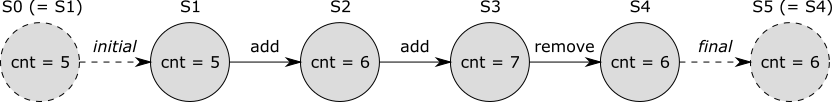
A transition with the initial label is added before the initial state, and a transition with the final label is added after the final state. This ensures that all states have an incoming and outgoing transition. These two added transitions are virtual, they don’t actually exist. They are added only for the benefit of print output. That is, they don’t affect the simulation behavior of the model, and are thus not part of the 'real' trace.
The added 'initial' virtual transition has no source state, and the added 'final' virtual transition has no target state. Since in the transition centric view every transition should have a source and a target state, we add the initial state (S1) as source state (S0) for the 'initial' transition, and the final state (S4) as target state (S5) for the 'final' transition. This way, every transition (whether virtual or real) has a source and target state, and fits the transition centric view. For the 'initial' and 'final' virtual transitions, the source and target states are thus the same (S0 = S1, S4 = S5).
The trace with added virtual 'initial' and 'final' transitions, and with the duplicates (S0 and S5) of the source and final states, is called the extended trace.
Every print declaration must specify what to print, using CIF expressions. These CIF expressions can for instance refer to variables from the CIF model. Since variables can change values, it is important to know in which state the expression is evaluated. In the transition centric view, we have two states to choose from, the pre/source state and the post/target state. The following variants are supported to specify what to print:
print EXPR;
print pre EXPR;
print post EXPR;
print pre EXPR post EXPR;The first variant has only one expression, which is printed in the post/target state. The third variant is identical, but explicitly indicates that the post/target state is used. The second variant also has a single expression, but is evaluated in the pre/source state. The fourth variant has two expression, one of which is evaluated in the pre/source state, and one of which is evaluated in the post/target state. The first three variants only print one piece of text per transition, while the fourth variant prints two pieces of text per transition.
Consider the following examples:
print "a";
print pre x post x;The first example prints a after each transition. The second example prints
the value of variable x as it was before the transition, as well as the
value of variable x as it is after the transition, for each transition.
The expressions that indicate what text to print may be of any type, and the
result of evaluating the expression is converted to a textual representation
that closely resembles the textual syntax of CIF. For string literals this
means that the text is escaped, and double quotes are added. If however the
result of the expression is a string typed value, then that string is used
'as is' (without quoting, and without escaping). Thus, consider the following
example:
print ["a\"b"];
print "a\"b";The first print declaration prints a list that contains a single string value, while the second print declaration prints the single string value directly. This results in the following printed output:
["a\"b"]
a"bThat is, in general string values are quoted and escaped, as is the case for the first example, where the result is a list. However, if the entire result is a string, as is the case with the second example, the string value is used 'as is', without quoting and without escaping.
It is possible to filter the transitions to which print declarations apply, by looking at the kind of the transitions (their labels). The following transition filters are available:
| Filter | Matches | Does not match |
|---|---|---|
|
All event transitions, including those for the |
All time and virtual transitions. |
|
All time transitions. |
All event and virtual transitions. |
e |
All transitions for event |
All time and virtual transitions, as well as all transitions for
'other' events (including those for the |
|
The single virtual initial transition. |
All event and time transitions, as well as the single virtual final transition. |
|
The single virtual final transition. |
All event and time transitions, as well as the single virtual initial transition. |
Transition filters may be combined, leading to a combined transition filter that matches if any of the individual transition filters matches. The individual filters must be separated by commas.
Transition filtering is optional. If no transition filter is supplied, the
default transition filter is used, which is initial, event, time. That is,
by default output is printed for all transitions, except for the final
virtual transition.
Consider the following examples:
print EXPR for e;
print EXPR for time, event;
print EXPR for initial, final;
print EXPR for machine1.start, machine2.start;
print EXPR;The first example prints only for transitions for event e. That is, time
transitions and virtual transitions, as well as transitions for all other
events, are filtered out. The second example prints only for event and time
transitions, and thus filters out the virtual transitions. The third example
prints only for the virtual transitions, and thus filters out all 'real'
transitions (the event and time transitions). The fourth example prints only
for transitions for the start events declared in machine1 and
machine2 (which could for instance be automata), and filters out time
transitions, virtual transitions, and transitions for all other events. The
fifth example does not specify a filter, and thus prints for the initial
virtual transition, as well as all event and time transitions, but excludes
the final virtual transition.
It is possible to filter the transitions to which print declarations apply, by looking at the pre/source and post/target states of the transitions. The following variants are supported for state filtering:
print EXPR when PRED;
print EXPR when pre PRED;
print EXPR when post PRED;
print EXPR when pre PRED post PRED;The first variant has only one predicate, which is evaluated in the post/target
state. The third variant is identical, but explicitly indicates that the
post/target state is used. For both these variants, text is only printed if the
post/target state satisfies the given predicate. That is, if the predicate
evaluated in the post/target state of the transition results in value true,
text may be printed. Otherwise, no text is printed for that transition.
The second variant also has a single predicate, but is evaluated in the pre/source state. Text is thus only printed if the pre/source state satisfies the given predicate.
The fourth variant has two predicates, one of which is evaluated in the pre/source state, and one of which is evaluated in the post/target state. Text is only printed if the pre/source state satisfies the first predicate, and the post/target state satisfies the second predicate. If either of the states does not satisfy its corresponding predicate, no text is printed for that transition.
Consider the following examples:
print "a";
print "b" when aut.loc;
print "c" when pre aut.loc;
print "d" when pre x mod 2 = 0 post x mod 2 = 1;The first example prints a after each transition, and does not restrict the
pre/source or post/target states. The second example only prints b for
transitions that end in location loc of automaton aut. The third
example only prints c for transitions that start in location loc of
automaton aut. The fourth example only prints d for transitions where
the value of variable x is even before the transition, and odd after the
transition.
State filtering is thus optional. If no pre/source state predicate is
specified, the default is true. Similarly, if no post/target state
predicate is specified, the default is true as well.
The transition and state filters are all optional. If however both a transition filter and a state filter are specified, they must both match in order for text to be printed. Consider the following examples:
print time for time when time > 3;
print x for e when pre x < 3 post x > 5;
print pre y post y when pre y = 5;For the first example, the value of variable time is printed after time
transitions, if after those time transitions the value of variable time is
strictly larger than three. For the second example, the value of variable x
is printed after transitions for event e if before such transitions the
value of variable x is strictly less than three, and after such transitions
the value of variable x is strictly larger than 5. For the third
example, the value of variable y is printed twice for all 'default'
transitions, once in the pre/source state, and once in the post/target state,
but only if the value of variable y before the transition is exactly five.
So if the condition over the pre/source state does not hold, the value of
variable y is not printed, not for the pre/source state, and also not for
the post/target state.
By default text is printed to the console, to the standard output stream, usually called 'stdout'. It is however possible to explicitly specify the file or special target to which the output is to be printed. Consider the following examples:
print ... file "txt_files/some_file.txt";
print ... file "../files/some_file.txt";For the first print declaration, the simulator will look for a txt_files
directory in the same directory as the CIF file, and print text to a file named
some_file.txt in that directory. For the second print declaration, the
simulator will look for a files directory in the parent directory of the
directory that contains the CIF file, and print text to a file named
some_file.txt in that files directory.
Files and directories are separated using slashes (/), regardless of the
used operating system. It is also allowed to use backslashes (\), which are
more common on Microsoft Windows operating systems, but they need to be escaped
as \\ for this to work, making it easier to use slashes (/) instead.
The following special non-file targets are supported:
-
":stdout": prints to the standard output stream. In Eclipse, the text ends up on the console, as black text. -
":stderr": prints to the standard error stream. In Eclipse, the text ends up on the console, as red text.
Besides these local file indications, CIF also supports global print file declarations, which influence the default, in case no local file or special target is specified.
Print file declarations can be specified in all components. That is, they can be specified in the top level scope of the specification, in groups and group definitions, as well as in automata and automaton definitions.
Print declarations can specify the file or special target to which text is to printed. If they don’t specify anything, the default is to print to the standard output stream, usually called 'stdout'. This default can be influenced by means of print file declarations, which act as a sort of global declaration of the file or special target. A typical print file declaration looks like this:
printfile "some_file.txt";It is possible to use relative (or absolute) paths for the files. For instance:
printfile "txt_files/some_file.txt";
printfile "../files/some_file.txt";For the first print file declaration, the simulator will look for a
txt_files directory in the same directory as the CIF file, and print text
to a file named some_file.txt in that directory. For the second print file
declaration, the simulator will look for a files directory in the parent
directory of the directory that contains the CIF file, and print text to a file
named some_file.txt in that files directory.
Files and directories are separated using slashes (/), regardless of the
used operating system. It is also allowed to use backslashes (\), which are
more common on Microsoft Windows operating systems, but they need to be escaped
as \\ for this to work, making it easier to use slashes (/) instead.
The following special non-file targets are supported:
-
":stdout": prints to the standard output stream. In Eclipse, the text ends up on the console, as black text. -
":stderr": prints to the standard error stream. In Eclipse, the text ends up on the console, as red text.
Print file declarations can (just as print declarations) be specified in all components. That is, they can be specified in the top level scope of the specification, in groups and group definitions, as well as in automata and automaton definitions. A print file declaration that is specified in a certain scope applies to that scope, as well as all child scopes that don’t have a print file declaration of their own. Additionally, print file declarations apply to all print declarations without local file declarations, in scopes to which the print file declarations apply.
For instance, consider the following CIF specification:
printfile "file1.txt";
print 5;
print 6 file "file2.txt";
group g:
printfile "file3.txt";
print 7;
print 8;
print 9 file "file4.txt";
group h:
printfile "file5.txt";
end
group i:
print 10;
end
endThe print declaration that prints 5 is declared in the top level scope of
the specification, and does not have a local file declaration. As such, the
print file declaration from the top level scope (file1.txt) applies to it.
The print declaration that prints 6 is declared in the same scope, but has
a local print file declaration (file2.txt). The local print file
declaration (file2.txt) overrides the print file declaration from the top
level scope (file1.txt).
Group g also has a print file declaration (file3.txt). This overrides
the print file declaration from the top level scope (file1.txt). The print
file declaration from group g (file3.txt) thus applies to the print
declarations that print 7 and 8, as they are declared in the same
scope, and don’t have local print file declarations. The print declaration that
prints 9 has a local print file declaration (file4.txt), and as such
the print file declaration from group g (file3.txt) does not apply to
it.
The print file declaration (file5.txt) from group g.h does not apply to
any print declarations. The simulator will open the file for writing, but no
text will be printed to the file. A warning is printed to the console, to
indicate the potential problem. However, no such warnings are ever printed for
special target 'stdout'.
Group g.i does not have a print file declaration, so the print file
declaration (file3.txt) from group g (the parent scope of group
g.i) applies to the print declaration that prints 10.
See also the Push print file declarations into print declarations CIF to CIF transformation.
In every scope (or component), in principle at most one print file declaration may be specified. The exception is that for a single scope, specified in multiple CIF files (when imports are used), if the print file declarations refer to the same target, they are merged. If however the two CIF files refer to different targets, this is still considered an error. It is also considered an error if two print file declarations are present in a single scope, in a single file, regardless of whether they refer to the same target or not. In the end, after processing imports, for every scope there must be a unique print file declaration, if one is declared at all.
If the same file or special target is used/specified multiple times, in different print file declarations or locally in print declarations, this is detected by the simulator. The simulator only opens a stream to the file or special target once, and prints to it all the output of all print declarations that apply to that file or special target. For instance, consider the following CIF specification:
print 5 file "some_file.txt";
print 6 file "some_file.txt";Even though both print declarations specify a file locally, they use the same file. The output of both print declarations is thus printed to the same file.
Once a CIF specification with print declarations is available, the simulator can be used to generate textual output. This page discusses the following simulation related topics:
If output is printed to files, those files are always overwritten for each simulation. That is, at the start of the simulation, the output file is removed if present. A new empty file is then created, to which the output is printed during the simulation.
Output is printed in a line-based fashion. That is, every time text is printed for a print declaration, the text is printed on a new line. If a single print declaration has two texts, one for the pre/source state and one for the post/target state, both texts are printed on new lines.
The simulator guarantees that once text is printed for a certain state, no text shall ever be printed during that same simulation, for previous states. That is, output text is ordered by 'increasing' states. This guarantee holds for file output. For the special targets standard output stream (stdout) and standard error stream (stderr), the output may get mixed, for instance on the Eclipse console.
The order in which text is printed for different print declarations that print text for the same state, is determined by the order in which the print declarations are specified in the CIF specification, from top to bottom. The order is determined per file or special target, after elimination of imports, component definition/instantiation, etc. A depth-first traversal of the component hierarchy is used, where the print declarations of components are considered before the print declarations of their children.
Print output is enabled by default. It can be disabled by reducing the types of normal console output using the Normal output option (Output category). Using that option it is also possible to disable all other forms of normal output, to be able to see only the print output on the console. Print output can also be disabled by changing the output mode to Error or to Warning, instead of Normal.
For text formatting, CIF features the fmt standard library function. This
page describes all the details of using that function. For more introductory
information and examples of the use of the fmt function for print output,
see the Text formatting tutorial.
The fmt function requires at least one argument, the format pattern. The
remaining arguments of the function are the values that can be inserted into
the format pattern, to allow variable output. For instance, consider:
fmt("%s %s", x, y)Here, "%s %s" is the format pattern, x is the first value, and y is
the second value.
The first argument, the format pattern, must be a string literal. That is, it
must be text between double quotes (").
The real usefulness of format patterns comes from the inclusion of the values
into the format pattern. The values can be included by inserting format
specifiers (e.g. %s) into the format pattern. Multiple values may be used
by including multiple format specifiers. The first format specifier includes
the first value, the second format specifier includes the second value, etc.
The result of fmt applied to it arguments is the text of the format
pattern, with the format specifiers replaced by their corresponding values.
Format specifiers can be customized to influence how their corresponding values are to be inserted. For instance, consider:
fmt("%s %.2e", x, y)Then, assuming variable x has value 3 and variable y has value
5.6, the result of the fmt function is 3 5.60e+00.
Format patterns support various types of format specifiers, each performing a different kind of conversion on its corresponding value. The following table lists the available conversions, the types of values that they support, and a short description of the output of the conversion:
| Conversion | Supported types | Output |
|---|---|---|
|
Either |
|
|
Same as |
|
|
Decimal integer notation. |
|
|
Hexadecimal integer notation, using |
|
|
Hexadecimal integer notation, using |
|
|
Computerized scientific notation, using |
|
|
Computerized scientific notation, using |
|
|
Decimal number notation. |
|
|
General scientific notation, using |
|
|
General scientific notation, using |
|
any type |
General textual representation. |
|
any type |
General textual representation, in upper case. |
For the %d, %x, and %X specifiers, int typed values are
supported, as are integer types with ranges (e.g. int[0..5]). The %s
and %S specifiers support values of any type.
The output of the %B specifier is identical to the output of the %b
specifier, where all letters in the output are converted to upper case letters.
This duality (lower case specifier conversion versus upper case specifier
conversion) is present in all conversions that can have letters in their
output.
Specifiers can be customized to influence the conversion of their corresponding values to text. The general syntax of specifiers is:
%[value_index$][flags][width][.precision]conversionAll specifiers start with a percentage character (%).
They are optionally followed by a value index. If the value index is specified,
it must be followed by a dollar sign ($). The value index is a positive
decimal integer indicating the position of the value in the value list. The
first value is referenced by 1$, the second by 2$, etc. Index zero and
indices starting with zero are not allowed.
The index is followed by optional flags. Flags are characters that modify the output, and may be specified in any order. Each flag may only be specified once per specifier. The set of valid flags depends on the conversion.
After the flags, an optional width may be specified. The width is a non-negative decimal integer indicating the minimum number of characters that should be included in the result, for that specific specifier.
After the width, a precision may optionally be specified. A precision is always
preceded by a dot (.). The precision is a non-negative decimal integer used
to restrict the number of characters. The specific behavior depends on the
conversion.
Specifiers always end with the character indicating the conversion to perform.
By default, format specifiers are processed in order. The first specifier then implicitly uses the first value, the second specifier implicitly uses the second value, etc. However, if an explicit value index is given, that explicit index indicates the value to use, and the specifier with the explicit index does not influence subsequent implicit indexing. That is, consider the following:
fmt("%s %1$s %3$f %d %f %1$s", 1, 2, 3.0);The first specifier (%s) does not specify an explicit index, and thus
implicitly uses the first value. The second specifier (%1$s) explicitly
specifies index 1 and thus uses the first value. The third specifier
(%3$f) explicitly specifies index 3 and thus uses the third value. The
fourth specifier (%d) is the second specifier to not explicitly specify an
index, and thus implicitly uses the second value. The fifth specifier (%f)
is the third specifier to not explicitly specify an index, and thus implicitly
uses the third value. Finally, the sixth specifier (%1$s) explicitly
specifies index 1, and thus uses the first value. The result of the
formatting is:
1 1 3.000000 2 3.000000 1
The following flags are available:
| Flag | b/B | d | x/X | e/E | f | g/G | s/S | Effect |
|---|---|---|---|---|---|---|---|---|
|
yes |
yes |
yes |
yes |
yes |
yes |
yes |
The result will be left-justified. |
|
no |
yes |
no |
yes |
yes |
yes |
no |
The result will always include a sign. |
(space) |
no |
yes |
no |
yes |
yes |
yes |
no |
The result will include a leading space for non-negative values. |
|
no |
yes |
yes |
yes |
yes |
yes |
no |
The result will be zero-padded. |
|
no |
yes |
no |
no |
yes |
yes |
no |
The result will include commas ( |
The first column shows the available flags, the minus (-), the plus
(+), the space, the zero (0), and the comma (,). The middle columns
indicate for each of the different conversions, whether the flags are
supported. The last column gives short descriptions of the effects of the
flags.
The - flag can be used to left-justify the text in case a
width is used, as the default
is to right-justify. It is supported by all format specifiers. The - flag
requires the use of a width, and can not be combined with the 0 flag.
The + flag can be used to always include a sign. It only applies to certain
numeric format specifiers. That is, by default non-negative numbers don’t have
a sign, and negative numbers start with a - character. By including the
+ flag, non-negative numbers start with a + character, and negative
numbers still start with a - character. The + and space flags can not
be combined.
The space flag can be used force a leading space to be included for
non-negative values. It only applies to certain numeric format specifiers. That
is, by default non-negative numbers don’t have a sign, and negative numbers
start with a - character. By including the space flag, non-negative numbers
start with a space character, and negative numbers still start with a -
character. The + and space flags can not be combined.
The 0 flag can be used to zero pad numbers, in case a
width is used, the text is
right-justified, and the text is shorter than the width. It only applies to
certain numeric format specifiers. The 0 flag requires the use of a width,
and can not be combined with left-justification (the - flag).
The , flag can be used to include commas (,) as grouping separators.
It only applies to certain numeric format specifiers. That is, by default
numbers are just a sequence of digits. By using the , flag, longer numbers
are placed in groups of thousands and the 'thousands separator' (the ,
character) occurs every three digits. For instance, 12345678 would then
become 12,345,678.
Further details on the effects of flags are given in the sections describing the individual conversions.
The width is a non-negative decimal integer indicating the minimum number of characters that should be included in the result, for that specific specifier. If no width is given, there is no minimum number of characters.
If the textual representation of the value is shorter than the width, the
text is right-justified. That is, the text will be padded by spaces to the
left of the text until the total number of characters equals the width. To
left-justify the text, use the - flag in combination with a width. This
results in padding with spaces to the right of the text.
If the 0 flag is specified, and the textual representation of the value is
shorter than the width, 0 padding is used (to the left, as the - flag
may not be used when the 0 flag is used). See the sections describing the
individual number related specifiers for further details.
If the text is longer than the width, the whole text is included in the result (it is not truncated), and the width essentially has no effect.
%b and %B specifiersThe %b and %B specifiers convert boolean values to text. The specifiers
only support boolean values. The specifiers support explicit indices, widths,
and the - flag. They don’t supports any of the other flags, and precisions.
The resulting text is constructed as follows:
-
Value
trueresults in the texttrue, and valuefalseresults in the textfalse. -
For the
%Bspecifier, the text is converted to upper case, i.e.TRUEandFALSErespectively. -
If a width is specified, and the resulting text so far is shorter than that width, spaces are added until the given width is reached. If the
-flag is given, spaces are added to the right, otherwise spaces are added to the left.
Here are some examples, assuming b has value true:
fmt("%b", b); // true
fmt("%B", b); // TRUE
fmt("_%10b_", b); // _ true_
fmt("_%-10b_", b); // _true _%d specifierThe %d specifier converts integer numbers to text, using decimal
representations of integers. The specifier only support integer values
(int typed values, and values of integer types with ranges, such as
int[0..5]). The specifier supports explicit indices, widths, and all flags.
It doesn’t support precisions.
The resulting text is constructed as follows:
-
The resulting text is initialized to the decimal representation of the absolute value of the integer number. It thus consists of only the digits
0through9. -
If the
,flag is given, thousand separators (,characters) are inserted as needed, for longer numbers. -
If the number is negative, it is prefixed with a
-character. -
If the number is non-negative, and the space flag is given, a space is added before the text.
-
If the number is non-negative, and the
+flag is given, a+character is added before the text. -
If a width is given, the text so far is shorter than the width, and the
0flag is given, then0characters are added before the other digits, and after any non-digit characters, until the desired width is reached. -
If a width is given, the text so far is shorter than the width, and the
-flag is given, then space characters are added before the result, until the desired width is reached. -
If a width is given, the text so far is shorter than the width, and neither the
0flag nor the-flag is given, then space characters are added after the result, until the desired width is reached.
Here are some examples, assuming x has value 12345 and y has value
-2345:
fmt("%d", x); // 12345
fmt("%,d", x); // 12,345
fmt("_%10d_", x); // _ 12345_
fmt("_%-10d_", x); // _12345 _
fmt("_%0,10d_", x); // _000012,345_
fmt("_%- 10d_", x); // _ 12345 _
fmt("_%- 10d_", y); // _-2345 _
fmt("_%-+10d_", x); // _+12345 _
fmt("_%-+10d_", y); // _-2345 _
fmt("_%3d_", x); // _12345_
%x and %X specifiersThe %x and %X specifiers convert integer numbers to text, using
hexadecimal representations of integers. The specifiers only support integer
values (int typed values, and values of integer types with ranges, such as
int[0..5]). The specifiers supports explicit indices, widths, and the -
and 0 flags. They don’t supports any of the other flags, and precisions.
The resulting text is constructed as follows:
-
The signed integer number in range [-2,147,483,648 .. 2,147,483,647] is first converted to an unsigned integer number in range [0 .. 4,294,967,295]. That is, for negative numbers, 232 is added.
-
The resulting text is initialized to the hexadecimal representation of the unsigned integer number. It thus consists the digits
0through9and lettersathroughf. -
For the
%Xspecifier, the text is converted to upper case, i.e. lettersathroughfare converted to lettersAthroughF. -
If a width is given, the text so far is shorter than the width, and the
0flag is given, then0characters are added before the result, until the desired width is reached. -
If a width is given, the text so far is shorter than the width, and the
-flag is given, then space characters are added before the result, until the desired width is reached. -
If a width is given, the text so far is shorter than the width, and neither the
0flag nor the-flag is given, then space characters are added after the result, until the desired width is reached.
Here are some examples, assuming a has value 5543 and b has value
-1:
fmt("%x", a); // 15a7
fmt("0x%x", a); // 0x15a7
fmt("0x%X", a); // 0x15A7
fmt("0x%X", b); // 0xFFFFFFFF
fmt("_%10x_", a); // _ 15a7_
fmt("_%-10x_", a); // _15a7 _
fmt("_%3x_", a); // _15a7_
%e and %E specifiersThe %e and %E specifiers convert real numbers to text, using
computerized scientific notation. The specifiers only support real
values. The specifiers supports explicit indices, widths, the -, +,
space, and 0 flags, and precisions. They don’t supports any of the other
flags.
Real numbers include a decimal mark, a symbol used to separate the integer
part from the fractional part of number, when written in decimal form. This
decimal mark is denoted by a dot (.).
The resulting text is constructed as follows:
-
The decimal mark of the real number is shifted to ensure that at most one non-zero digit occurs to the left of it. That is, for real numbers
0.012,0.12,1.2,12.0, and120.0, the decimal mark is shifted -2, -1, 0, 1, and 2 digits to the left, respectively. This results in the following real numbers:1.2,1.2,1.2,1.2, and1.2. For zero, the decimal mark is not shifted. -
The single decimal digit before the decimal mark is included in the result. If there is no digit before the decimal mark (in case the real number is zero), a single
0digit is included in the result. -
If the precision is specified and is not zero, or if the default precision is used, a dot (
.) is added after the single digit. -
The digits after the decimal mark are added after the dot. Exactly 'precision' digits will be added. If no precision is specified, it defaults to
6digits after the dot. If not enough digits are available after the dot, additional0characters are added after them, to reach the desired precision. If too many digits are available after the dot, digits are removed from the right until the desired precision is reached. Rounding using the 'half up' algorithm is used to ensure correct results in case digits are removed. -
If the
%especifier is used, anecharacter is added to the end. If the%Especifier is used, anEcharacter is added to the end. -
A sign character is added after that. That is, if the decimal mark was shifted a negative number of digits to the left, a
-character is added, otherwise a+character is added. -
The number of digits that was shifted is added as a decimal number, at the end. At least two decimal digits are added, so if the number of digits that was shifted can be represented using a single decimal digit, a
0is added between theeorEcharacter and the number of digits that was shifted. -
If the real number is negative, the text is prefixed with a
-character. -
If the real number is non-negative, and the space flag is given, a space is added before the text.
-
If the real number is non-negative, and the
+flag is given, a+character is added before the text. -
If a width is given, the text so far is shorter than the width, and the
0flag is given, then0characters are added before the other digits, and after any non-digit characters, until the desired width is reached. -
If a width is given, the text so far is shorter than the width, and the
-flag is given, then space characters are added before the result, until the desired width is reached. -
If a width is given, the text so far is shorter than the width, and neither the
0flag nor the-flag is given, then space characters are added after the result, until the desired width is reached.
Here are some examples, assuming a has value 12345.6789 and b has
value -0.00002345678:
fmt("%e", a); // 1.234568e+04
fmt("%E", a); // 1.234568E+04
fmt("%.3e", a); // 1.235e+04
fmt("%.3e", b); // -2.346e-05
fmt("_%20e_", a); // _ 1.234568e+04_
fmt("_%-20e_", a); // _1.234568e+04 _
fmt("_%5e_", a); // _1.234568e+04_
fmt("_%020e_", a); // _000000001.234568e+04_
fmt("_%-+20e_", a); // _+1.234568e+04 _
fmt("_%-+20e_", b); // _-2.345678e-05 _
fmt("_%- 20e_", a); // _ 1.234568e+04 _
fmt("_%- 20e_", b); // _-2.345678e-05 _%f specifierThe %f specifier converts real numbers to text, using a decimal number
notation. The specifier only supports real values. The specifier supports
explicit indices, widths, all flags, and precisions. That is, all features of
format specifiers are supported.
Real numbers include a decimal mark, a symbol used to separate the integer
part from the fractional part of number, when written in decimal form. This
decimal mark is denoted by a dot (.).
The resulting text is constructed as follows:
-
The decimal digits before the decimal mark are included in the result. If there are no digits before the decimal mark, a single
0digit is included in the result. -
If the
,flag is given, thousand separators (,characters) are inserted as needed, for longer numbers. -
If the precision is specified and is not zero, or if the default precision is used, a dot (
.) is added after the digits. -
The digits after the decimal mark are added after the dot. Exactly 'precision' digits will be added. If no precision is specified, it defaults to
6digits after the dot. If not enough digits are available after the dot, additional0characters are added after them, to reach the desired precision. If too many digits are available after the dot, digits are removed from the right until the desired precision is reached. Rounding using the 'half up' algorithm is used to ensure correct results in case digits are removed. -
If the real number is negative, the text is prefixed with a
-character. -
If the real number is non-negative, and the space flag is given, a space is added before the text.
-
If the real number is non-negative, and the
+flag is given, a+character is added before the text. -
If a width is given, the text so far is shorter than the width, and the
0flag is given, then0characters are added before the other digits, and after any non-digit characters, until the desired width is reached. -
If a width is given, the text so far is shorter than the width, and the
-flag is given, then space characters are added before the result, until the desired width is reached. -
If a width is given, the text so far is shorter than the width, and neither the
0flag nor the-flag is given, then space characters are added after the result, until the desired width is reached.
Here are some examples, assuming a has value 12345.6789 and b has
value -0.00002345678:
fmt("%f", a); // 12345.678900
fmt("%f", b); // -0.000023
fmt("%.3f", a); // 12345.679
fmt("_%20f_", a); // _ 12345.678900_
fmt("_%-20f_", a); // _12345.678900 _
fmt("_%-,20f_", a); // _12,345.678900 _
fmt("_%5f_", a); // _12345.678900_
fmt("_%020f_", a); // _0000000012345.678900_
fmt("_%-+20f_", a); // _+12345.678900 _
fmt("_%-+20f_", b); // _-0.000023 _
fmt("_%- 20f_", a); // _ 12345.678900 _
fmt("_%- 20f_", b); // _-0.000023 _
%g and %G specifiersThe %g and %G specifiers convert real numbers to text, using general
scientific notation. The specifiers only support real values. The specifiers
supports explicit indices, widths, all flags, and precisions. That is, all
features of format specifiers are supported.
Real numbers include a decimal mark, a symbol used to separate the integer
part from the fractional part of number, when written in decimal form. This
decimal mark is denoted by a dot (.).
If the real number is is greater than or equal to 10-4 but
less than 10precision, the result is as %f. Otherwise, the
result is as %e and %E, for %g and %G respectively. However,
the total number of
significant digits
of the
result is equal to the precision of the %g or %G specifier, and
defaults to 6 if not specified. If the specified precision is 0, it is
taken to be 1 instead.
Here are some examples, assuming a has value 12345.6789 and b has
value -0.00002345678:
fmt("%g", a); // 12345.7
fmt("%g", b); // -2.34568e-05
fmt("%G", b); // -2.34568E-05
fmt("%.3g", a); // 1.23e+04
fmt("_%20g_", a); // _ 12345.7_
fmt("_%-20g_", a); // _12345.7 _
fmt("_%-,20g_", a); // _12,345.7 _
fmt("_%5g_", a); // _12345.7_
fmt("_%020g_", a); // _000000000000012345.7_
fmt("_%-+20g_", a); // _+12345.7 _
fmt("_%-+20g_", b); // _-2.34568e-05 _
fmt("_%- 20g_", a); // _ 12345.7 _
fmt("_%- 20g_", b); // _-2.34568e-05 _
%s and %S specifiersThe %s and %S specifiers convert any value to text. The specifiers
support values of any type. The specifiers supports explicit indices, widths,
and the - flag. They don’t supports any of the other flags, and precisions.
The resulting text is constructed as follows:
-
If the value has a
stringtype, the value of that string is used as is, without escaping and double quoting. Otherwise, the value is converted to a textual representation closely resembling the CIF textual syntax (ASCII syntax), with string values surrounded by double quotes, and with special characters (tabs, new lines, double quotes, and backslashes) escaped. -
For the
%Sspecifier, the text is converted to upper case, i.e. lettersathroughzare converted to lettersAthroughZ. -
If a width is specified, and the resulting text so far is shorter than that width, spaces are added until the given width is reached. If the
-flag is given, spaces are added to the right, otherwise spaces are added to the left.
Here are some examples, assuming x has value "aBcD":
fmt("%s", x); // aBcD
fmt("%S", x); // ABCD
fmt("_%10s_", x); // _ aBcD_
fmt("_%-10s_", x); // _aBcD _As indicated above, string typed values are of special interest. For
instance, consider the following examples:
fmt("a %s b", ("some \\ text", 6)); // a ("some \\ text", 6) b
fmt("a %s b", "some \\ text"); // c some \ text dThe first example has a tuple as value, with a string and an integer number.
The output of this example is a ("some \\ text", 6) b. Note how the string
in the tuple is included in the output with double quotes around it, and how
the escaped backslash is also escaped in the resulting text.
The second example has a value that is a string directly (e.g. not contained in
a tuple or some other container). This mapping results in c some \ text d.
Note how the string is included in the output 'as is', i.e. it is not
surrounded by double quotes, and the backslash is not escaped.
In general, when using a %s specifier, string values are double quoted and
escaped. If however the entire value is a string, then that string is used
'as is' (without quoting, and without escaping).
Also of special interest are real values. The number of digits after the decimal point can vary. For instance, consider the following examples:
fmt("a %s b", 1 / 3); // a 0.3333333333333333 b
fmt("c %s d", 1 / 2); // c 0.5 dFor more control over the number of digits after the decimal point, use one of the floating point number format specifiers: %e, %E, %f, %g, or %G.
Double quote terminate string literals, and thus also a format pattern, as
format patterns are string literals. It is therefore not possible to include
a double quote in the text of a format pattern without escaping it. That is,
use \" inside a format pattern to include a single double quote. There are
other escape sequences as well. Use \\ to include a single backslash
(\), \n to include a single new line (to continue on a new line), and
\t to include a tab character (for alignment).
Format specifiers start with a percentage character (%). If a percentage
character is to be included as a percentage character instead of being
interpreted as a format specifier, it needs to be escaped as well. That is,
to include a percentage character as a percentage character, use %% in
the format pattern.
For instance, the format pattern "a\"b\nc\td\\e%%f" results in the
following text:
a"b
c d\e%fThe format pattern is automatically checked for unused values. That is, if a value is not used in the format pattern, there is no use in specifying it, and a warning will indicate this.
SVG visualizer
The CIF simulator supports several forms of output. By default, simulation results, such as the current state, are printed to the console. While this provides useful information, it is not easy to decipher the precise state of a (sub-)system. Also, it does not give a graphical overview of the current state of the system.
The simulator however, also supports SVG visualization, which allows the user to make an image of the system, and have that image be updated by the simulator during simulation, based on the current state of the system. This allows the user to see changes in the state of the system, in a graphical representation of that system. This makes it much easier to get a global overview of the system during simulation. Since the user makes the image, the representation directly corresponds to the way the user sees the system.
Documentation
Examples
Below is a list of available examples of SVG visualizations, which show some often used SVG attributes, as well as some tips and tricks on how to handle common challenges. The following examples are available:
Before we go into any details about SVG visualization, let’s first look at an example. Here, we use a trivial example, which nonetheless serves several purposes:
-
It gives a quick overview of what the idea of SVG visualization is all about, and what it looks like.
-
It shows how to use SVG visualization with the CIF simulator.
-
It shows the two alternatives to simulation: via the options dialog, and by using a ToolDef script.
Note that it is not necessary to fully understand what exactly is going on, or how it works. Those details should become clear after reading the remaining pages of the documentation.
In an Eclipse project or directory, create a new CIF file named lamp.cif:
svgfile "lamp.svg";
automaton lamp:
cont t der 1.0;
location Off:
initial;
edge when t >= 1.0 do t := 0.0 goto On;
location On:
edge when t >= 2.0 do t := 0.0 goto Off;
svgout id "lamp" attr "fill" value if Off: "gray" else "yellow" end;
endThis file describes not only the behavior of the lamp using a CIF automaton, but also contains a CIF/SVG declaration, which specifies the connection between the behavioral CIF specification and the SVG image.
Next, we’ll create an SVG image.
Start
Inkscape,
Select
Document Properties…
from the
File
menu, to open the
Document Properties
window. On the
Page
tab, set the
Units
to
px,
the
Width
to 75.00, and
the height to 100.00. It is recommended to always
set the size of the image,
before adding any shapes or text labels.
Next, select the circle tool, by clicking on the circle in the Toolbox on the left side of the application. Draw a circle on the canvas. It should look something like this:
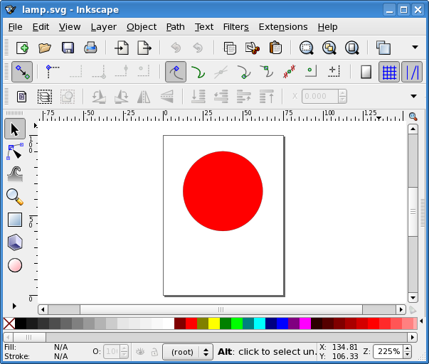
Right click the circle and choose
Object Properties.
The
Object Properties
window will appear. Change the
Id
of
the circle to lamp and click the
Set
button. Save the image
as lamp.svg, in the same directory as the lamp.cif file.
Right click the lamp.cif file and choose
Simulate CIF specification…
to start the CIF simulator. An
options dialog appears. In this case the defaults suffice, so click
OK
to start the simulation. Initially, the visualization looks as
follows:
Using the GUI input, click the button for time delay and then the button for tau. After performing these two transitions, the visualization should look as follows:
As you can see, the lamp is gray while it is off, and yellow while it is on. Close the GUI input to terminate the simulator. You may also close the visualization window.
Now restart the simulator. In the Simulator category, set the Simulation end time option to Finite end time. You can leave the default value for End time. In the Input category, set the Input mode option to Automatic input mode. In the Output category, enable the Frame rate option and keep the default frame rate value. Click OK to start the simulation again. This time, the simulator automatically chooses transitions. Furthermore, real-time simulation is enabled, where the model time is interpreted in seconds, and the visualization is regularly updated. Using these options, SVG visualization essentially turns into an SVG movie of the simulation of a flashing lamp. Simulation will automatically stop after ten seconds, the default simulation end time. Once simulation terminates, you may close the visualization window.
While the option dialog is useful for configuring simulation options, it is
often easier to use a ToolDef file to
script the execution of the CIF simulator.
Create a new file named lamp.tooldef, in the same directory as the other
files, and give it the following content:
from "lib:cif" import *;
cifsim(
"lamp.cif",
"-t 10",
"-i auto",
"--frame-rate=20",
);Don’t forget to save the file. Right-click the lamp.tooldef file and
choose
Execute ToolDef
to execute the ToolDef script. This script
uses the exact same options as we manually configured in the option dialog, in
the previous section.
The SVG visualization feature uses Scalable Vector Graphics (SVG) images. SVG is a widely-deployed royalty-free standard for two-dimensional vector graphics, developed by the World Wide Web Consortium (W3C). SVG images consist of three types of objects: vector graphic shapes (rectangles, circles, etc.), raster images, and text. The benefit of vector images formats over raster image formats, is that raster images are created with a fixed size, while vector images contain a description of the image and can be rendered at any size without loss of quality.
Multiple versions of the SVG standard exist. The CIF simulator uses the free and open source Apache Batik SVG Toolkit to render SVG images. Batik supports version 1.1 of the SVG specification.
SVG image files are stored in an XML-based file format. This means that they can be edited with any text editor. However, it is often more convenient to edit them with a drawing program that supports vector graphics, such as Adobe Illustrator or Inkscape. Most modern web browsers also support SVG images.
Since SVG images are essentially XML files, we get all the benefits of XML for free. One of those benefits is that XML files represent tree structures, which can be easily manipulated by applications. This is essential for the CIF simulator. During initialization, the CIF simulator loads the SVG image file that the user provided, and subsequently has access to the XML tree. It then uses the aforementioned Batik toolkit to draw the SVG image represented by the XML tree. Once the simulator starts taking transitions and updates its state, it can use the information from the state to modify the XML tree. Changes to the XML tree then result in an updated SVG image, the next time the image is rendered again.
In order to be able to modify particular objects (shapes, text labels, etc.) of
the SVG image, the simulator should be able to identify the objects that make
up the image. Here we once again reap the benefits of XML. All nodes (called
elements) in the XML tree can have an id attribute that specifies the
id (also called name or identity) of the element. As such, all SVG objects can
be identified using their unique id. The
SVG element id section of the
CIF/SVG output mappings page further explains the
use of SVG element ids.
The website of Jakob Jenkov has a very nice SVG Tutorial.
SVG images can best be edited with a drawing program that supports vector graphics. One such program is Inkscape, a free and open source vector graphics editor that uses SVG as its native file format, and is available for many platforms, including Microsoft Windows, macOS, and Linux. In this documentation, we’ll use Inkscape to create and edit SVG images.
It is beyond the scope of this document to explain how Inkscape works. For that, see the Inkscape website. Here is a screenshot of the Inkscape interface:
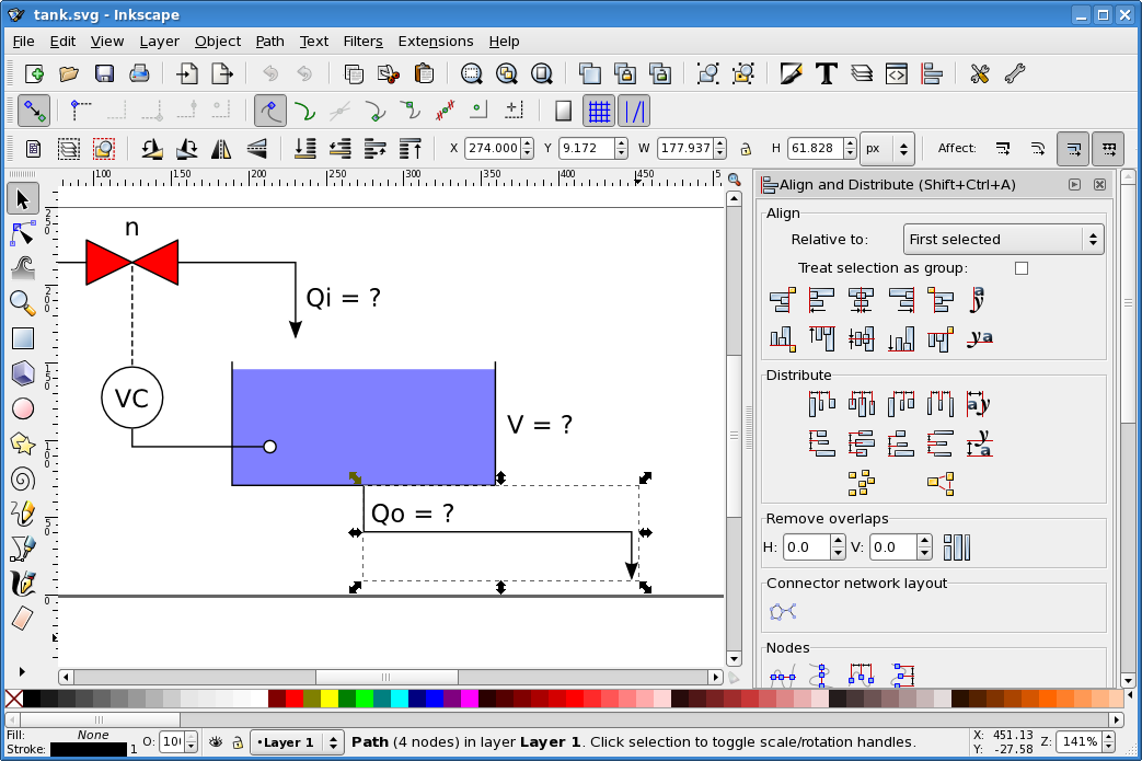
As described on the page about SVG, every SVG object has an id. To change the id of an object in Inkscape, right click on the object, and choose Object Properties. The Object Properties window will appear, which looks like this:
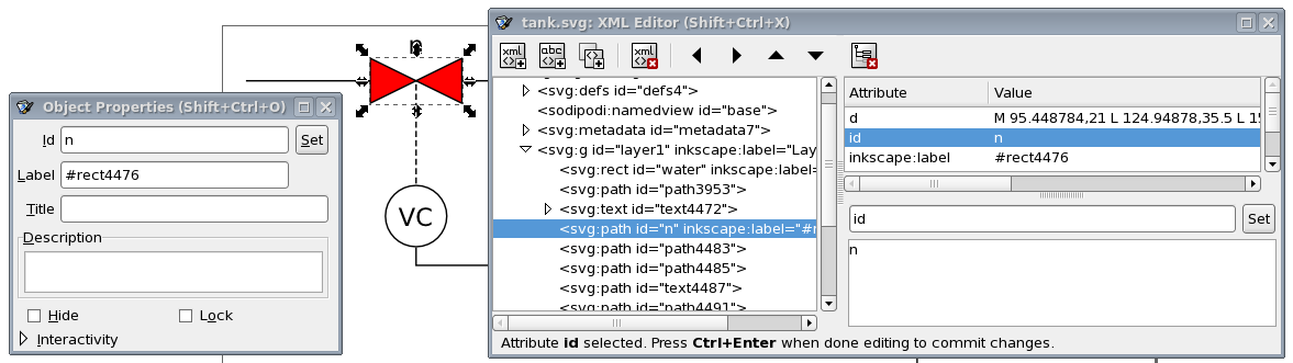
In this window, you can change the object’s id, by entering a new id in the Id field, and clicking the Set button.
Inkscape also features an XML editor, that can be used to view and edit the underlying XML representation of the SVG image. The screenshot above also shows Inkscape’s XML Editor window, which can be opened via the XML Editor… item in the Edit menu. The XML editor can be useful to find out the exact structure of the XML tree, and to see the precise definitions that were used to represent the objects that you created on Inkscape’s canvas.
It is recommended to always set the correct size of the image, before adding any shapes or text labels. To do this, select Document Properties… from the File menu, to open the Document Properties window. On the Page tab, we recommend to set the Units to px. You can then enter the Width and Height of the image.
By default, Inkscape always adds a layer to new images. When changing the size
of the image as described above, this layer gets a transform attribute
that can cause all kinds of trouble later on. There are several ways to get
rid of this transform attribute of the layer:
-
Select Layers… from the Layer menu to show the Layers panel. In that panel, select Layer 1 by clicking on it. Then click the Delete the current layer button to remove the selected layer.
-
Use the XML Editor to select the layer (
<svg:g id="layer1"… node). Then click the Delete node button at the top of the XML Editor window to remove the layer. Alternatively, after selecting the layer, press the Delete key on the keyboard to delete the selected layer. -
Use the XML Editor to select the layer (
<svg:g id="layer1"… node). Then, on the right, select thetransformattribute by clicking on it. Then click the Delete attribute button at the top of the XML Editor window to remove the attribute.
The first two approaches remove the layer, the third approach keeps the layer
and only removes the transform attribute.
Alternatively, there is also a way to avoid the transform attribute from
being added in the first place. Instead of using the
Document Properties
window to change the size of the image, do
the following:
-
Use the XML Editor to select the entire image (
<svg:svg… node). -
Select the
widthattribute on the right, by clicking on it. -
Change the value in the text area at the lower right corner of the window.
-
Click the Set button to save the new width value. Alternatively, after typing the new value, press Ctrl+ENTER to save the new width value.
-
Repeat for the
heightattribute.
The coordinate system used by Inkscape uses the lower left corner of the canvas as origin, while the underlying SVG representation uses the upper left corner of the canvas as origin. Also, Inkscape uses x and y coordinates of objects relative to the outside of their border (called stroke in Inkscape), while SVG uses x and y coordinates of objects relative to the middle of their border. These are two most commonly encountered differences between Inkscape and SVG. See the tank example for some tips and tricks regarding the difference in coordinate systems.
When using the Inkscape text tool, select the tool, and left click once on the canvas to add a text label. Once you added it, start typing text.
Inkscape also allows you to select the text tool, left click anywhere on the
canvas, drag the mouse pointer to another position, and only then release the
left mouse button. This creates a text area, where text is automatically
wrapped to multiple lines, so that it stays within the bounds of the text area.
This feature uses SVG flowRoot elements. These elements are defined in
version 1.2 of the SVG standard, which is currently still a working draft.
These elements are not supported by the CIF simulator, which only supports
version 1.1 of the SVG standard.
Using an SVG image with a flowRoot or other unsupported SVG feature,
results in the following error when the SVG file is
opened in Eclipse:
ERROR: SVG image file "some_image.svg" is not an SVG file, is an invalid SVG file, or contains unsupported SVG features.
CAUSE: invalid.elementThe connection between the state of the CIF specification and the SVG image can be specified by using CIF/SVG declarations (sometimes also called SVG declarations, for simplicity). Such declarations can be specified directly in the CIF specification. CIF/SVG declarations are an extension to the CIF language, and can only be used to couple the model to the image. They don’t influence the behavior of the model itself.
The CIF text editor provides full integration for the CIF/SVG declarations extension, complete with syntax highlighting, background validation, etc.
The following types of CIF/SVG declarations are available:
-
SVG file declarations: Specifies which SVG image file to use.
-
CIF/SVG copy declaration: Specifies that a part of the SVG image should be copied.
-
CIF/SVG move declaration: Specifies that a part of the SVG image should be moved.
-
CIF/SVG output mappings: Specifies how to update a certain property of an element of the SVG image.
-
CIF/SVG input mappings: Specifies how interaction with the SVG image affects simulation.
Before any other CIF/SVG declarations can be specified, you need to indicate to which SVG image (file) they apply, using an SVG file declaration. A typical SVG file declaration looks like this:
svgfile "some_file.svg";The SVG files are declared based on their file names. If possible, it is recommended to use the same file name for the CIF specification and for the SVG image, only with different file extensions. This way, it is easy to see which images goes with which CIF specification.
It is possible to use relative (or absolute) paths for the SVG files. For instance:
svgfile "svg_files/some_file.svg";
svgfile "../images/some_file.svg";For the first SVG file declaration, the tools will look for an svg_files
directory in the same directory as the CIF file, and for a some_file.svg
file in that svg_files directory. For the second SVG file declaration, the
tools will look for an images directory in the parent directory of the
directory that contains the CIF file, and for a some_file.svg file in that
images directory.
Files and directories are separated using slashes (/), regardless of the
used operating system. It is also allowed to use backslashes (\), which are
more common on Microsoft Windows operating systems, but they need to be escaped
as \\ for this to work, making it easier to use slashes (/) instead.
CIF/SVG file declarations (and all 'other' CIF/SVG declarations) can be specified in all components. That is, they can be specified in the top level scope of the specification, in groups and group definitions, as well as in automata and automaton definitions. An SVG file declaration that is specified in a certain scope applies to that scope, as well as all child scopes that don’t have an SVG file declaration of their own. Additionally, all 'other' CIF/SVG declarations (such as SVG output mappings) may include a local SVG file declaration, that only applies to that specific CIF/SVG declaration.
For instance, consider the following CIF specification:
svgfile "file1.svg";
svgout id "a" attr "b" value 5;
svgout id "c" attr "d" value 6 file "file2.svg";
group g:
svgfile "file3.svg";
svgout id "e" attr "f" value 7;
svgout id "g" attr "h" value 8;
svgout id "i" attr "j" value 9 file "file4.svg";
group h:
svgfile "file5.svg";
end
group i:
svgout id "k" attr "l" value 10;
end
endThe mapping for the SVG element with id a is declared in the top level
scope of the specification, and does not have a local SVG file declaration.
As such, the SVG file declaration from the top level scope (file1.svg)
applies to it. The mapping for the SVG element with id b is declared in
the same scope, but has a local SVG file declaration (file2.svg). The local
SVG file declaration (file2.svg) overrides the SVG file declaration from
the top level scope (file1.svg).
Group g also has an SVG file declaration (file3.svg). This overrides
the SVG file declaration from the top level scope (file1.svg). The SVG
file declaration from group g (file3.svg) thus applies to the
mappings for ids e and g, as they are declared in the same scope, and
don’t have local SVG file declarations. The mapping for SVG element id i
has a local SVG file declaration (file4.svg), and as such the SVG file
declaration from group g (file3.svg) does not apply to it.
The SVG file declaration (file5.svg) from group g.h does not apply to
any mappings. The simulator will show the image, but the image will not change
during simulation. A warning is printed to the console, to indicate the
potential problem.
Group g.i does not have an SVG file declaration, so the SVG file
declaration (file3.svg) from group g (the parent scope of group
g.i) applies to the mapping for SVG element id k.
See also the Push SVG file declarations into other CIF/SVG declarations CIF to CIF transformation.
Every CIF/SVG declaration that is not itself an SVG file declaration, requires an SVG file declaration, in its scope, in one of its ancestor scopes, or locally in that CIF/SVG declaration itself.
In each scope, there may be at most one SVG file declaration.
In every scope (or component), in principle at most one SVG file declaration may be specified. The exception is that for a single scope, specified in multiple CIF files (when imports are used), if the SVG file declarations refer to the same image file, they are merged. If however the two CIF files refer to different image files, this is still considered an error. It is also considered an error if two SVG file declarations are present in a single scope, in a single file, regardless of whether they refer to the same image file or not. In the end, after processing imports, for every scope there must be a unique SVG file declaration, if one is declared at all.
If the same SVG image file is specified multiple times, in different SVG file declarations, this is detected by the simulator, and the image will only be shown once. For instance, consider the following CIF specification:
svgout id "..." attr "..." value 5 file "some_file.svg";
svgout id "..." attr "..." value 6 file "some_file.svg";Even though both output mappings specify an SVG file locally, they use the same file. The SVG image will thus only be shown once, and both mappings apply to the same image.
For each update of a single attribute of an element in the SVG image, an output mapping is needed. An output mapping essentially defines a connection between the CIF specification and the SVG image, for updating that specific attribute of that specific element.
Assume we have the following CIF specification:
cont pos der 1.0;Where variable pos is the position of some object, say a box. Then the
following output mapping:
svgout id "box" attr "x" value pos;Keeps the value of the x attribute of the SVG element with id box equal
to the value of continuous variable pos.
The general syntax of CIF/SVG output mappings is:
svgout id <id> attr <attr> value <value>;
svgout id <id> attr <attr> value <value> file <file>;
svgout id <id> text value <value>;
svgout id <id> text value <value> file <file>;The svgout keyword is followed by a specification of an SVG element
id. Every output mapping must
specify the id of an SVG
element, and an SVG element with that id must exist in the SVG image. The
id indicates the element for which an attribute or text is to be updated.
The id is followed by a specification of what part of the SVG element is to
updated. That is, either an
attribute or
text (label) is updated.
After that, the value of the attribute or text (label) is specified.
In the syntax examples above, we see that it is also allowed to declare an optional local SVG file declaration, that only applies to that specific output declaration.
Every output mapping needs to specify the id of the SVG element to update. The id is checked, to make sure an SVG element with that id actually exists in the SVG image.
Only valid SVG names may be used as ids. Valid SVG names start with a letter
(a to z, A to Z), an underscore (_), or a colon (:),
and may be followed by more of the same characters, as well as dashes (-),
dots (.), and numbers (0 to 9).
Ids must be put between double quotes. For instance, to use some-name as
id, it must be written as "some-name".
Instead of using a hard coded SVG element id, it is also allowed to use an
expression that when evaluated results in the SVG element id. Such an
expression must evaluate to a string typed value, and must be statically
evaluable (must not refer to variables that can change value during simulation,
etc). For instance:
// Hard coded SVG element id.
svgout id "box" attr "width" value ...;
// Computed SVG element id.
const string c = "bo";
svgout id c + "x" attr "width" value ...;The first output mapping applies to the SVG element with the id box. The
box id is hard coded into the output mapping. The second
output mapping uses the expression c + "x" to specify the SVG element id.
Once the expression is evaluated (its value is computed), this results in the
string typed value "box". As such, the second mapping applies to the
SVG element with id box as well.
The expressions may also refer to for instance algebraic parameters of automaton definitions. Since different values can be given to the parameters for each instantiation, this allows the SVG element id to vary for the different instantiations of the automaton definition. This particular usage allows for reuse and scalable solutions. The lamps example and workstation example are good examples of this usage. This usage is often combined with CIF/SVG copy declarations and CIF/SVG move declarations.
Every output mapping needs to specify the name of the attribute of the SVG
element to update (or text, see the
Text labels section).
Similarly to specifying ids, attribute names must be valid SVG names. They also
need to be put between double quotes. Unlike SVG element ids, it is not
possible to use expressions to specify attribute names. That is, only hard
coded names can be used to specify attribute names.
It is not allowed to change the ids of SVG elements, as it could lead to
duplicate or missing ids. As such, output mappings for the id attribute
(in any casing) are explicitly not supported. Similarly, changing the style
attribute (in any casing) using an output mapping is explicitly not supported,
to avoid conflicting style changes. See also the
SVG presentation attributes vs CSS style attributes section for more
information about the style attribute.
The supported attributes for an SVG element depend on what kind of element it
is. For instance, a rect element can have an x and y position, a
width and height, a fill color, etc. A g element (a group)
however, does not support those position attributes. It is beyond the scope of
this document to go into more detail. The software however, will warn about
using attribute names that are not supported according to the SVG standard (to
catch simple spelling mistakes), and specifying attributes on elements that
don’t support them. Consult the official
SVG specification
for further details. The
examples showcase several
commonly used attributes as well.
SVG uses two kinds of attributes: SVG presentation attributes, and CSS style attributes. For instance, in the following partial SVG image:
<rect fill="red" id="rect1" width="25" height="25" x="65" y="5"/>
<rect style="fill:red;" id="rect2" width="25" height="25" x="15" y="5"/>Rectangle rect1 uses the SVG presentation attribute fill to specify the
fill color the rectangle. Rectangle rect2 uses the CSS style attribute
fill to specify the fill color the rectangle. The SVG presentation
attributes are all direct attributes of the SVG element. CSS style attributes
on the other hand, are always part of the SVG presentation attribute style.
CSS stands for Cascading Style Sheets, and it is a style sheet language used for describing the look and formatting of a document. It’s best known for its use in styling web pages written in HTML. Like SVG, CSS is an international standard developed and maintained by the World Wide Web Consortium (W3C). SVG reuses the CSS standard for its CSS style attributes. The most commonly used attributes for certain elements are also available in the SVG standard as SVG presentation attributes. Furthermore, SVG adds additional presentation attributes not found in CSS.
If an attribute is specified on an element using both an SVG presentation
attribute, and a CSS style attribute, the CSS style attribute usually takes
precedence. The output mappings handle all of this automatically and
transparently. That is, you just specify the attribute name in the header of
the output mapping, and the simulator makes sure the proper attribute is
update, regardless of whether it is an SVG presentation attribute, or a CSS
style attribute. It is explicitly not supported to change the style
attribute directly (using an output mapping), in order to avoid conflicting
style changes when other output mappings update CSS style attributes that are
part of that same style SVG presentation attribute.
Changing the text of text labels is a special case, as text is not stored in attributes. Consider the following partial SVG image, which contains a text label (created using Inkscape, and with some of the irrelevant details omitted):
<text x="5" y="5" id="text1" style="font-size:16px;">
<tspan x="5" y="5" id="tspan2">
The actual text.
</tspan>
</text>Here we see a text element with id text1, which contains a tspan
element with id tspan2. The tspan element contains some text. To change
the text of this text label, use one of the following mappings:
svgout id "text1" text value ...;
svgout id "tspan2" text value ...;Here, instead of the attr keyword followed by the name of the attribute, we
simply specify the text keyword. We can either use the id of the text
element, or the id of the tspan element. More precisely, we can use the id
of an element that contains text (such as the tspan element in our
example), or an element (such as the text element in our example) that has
a single child, which contains text, or an element that has a single child,
which has an single child, which contains text, etc.
In practice, it is usually the easiest to use the
Object Properties
dialog of Inkscape, to get the
properties of the text label. The
Id
that is then shown, is the id of the text element.
Note that Inkscape can create
text areas (SVG flowRoot elements),
which are not supported by the CIF tooling.
In order for an output mapping to be able to update attributes or text labels, it needs a value. The simple output mapping example already showed how a value can be specified. This section further explains the details of the specification of such values.
The value keyword is followed by an expression. This expression may
for instance be a literal value, such as 1, true, 1.0,
"some text", or [1, 2]. At first, it might not seem useful to use a
literal as a value for an output mapping, since the mapping will then produce
the same value every time it is applied. However, the
rate example shows why this can in fact be
very useful.
The expressions however, may also contain references to variables (discrete,
continuous, or algebraic), functions, constants, locations, etc. For instance,
we could use the value of a continuous variable and multiply it by two, by
using x * 2 as expression, assuming that the continuous variable is named
x. Since we may refer to the state of
the CIF specification, the value of the expression can change as the simulation
continues, resulting in different values being mapped to the image.
The expressions can also include if expressions, which are particularly
powerful in this context. Using if expressions, a different value can be
used for several different conditions. See the
workstation example for an example of using
if expressions in an output mapping.
The value expression of an output mapping may be of any type. The result of
evaluating the expression is converted to a textual representation that closely
resembles the textual syntax of CIF, before using it to set the value of an
attribute, or the text of a text label. For string literals this means that the
text is escaped, and double quotes are added. If however the result of the
expression is a string typed value, then that string is used 'as is'
(without quoting, and without escaping). Thus, consider the following examples:
svgout id "..." attr "..." value ["a\"b"];
svgout id "..." attr "..." value "a\"b";The value of the first output mapping is a list that contains a single string value, while the value of the second output mapping is a string value directly. This results in the following texts being used as values of the attributes:
["a\"b"]
a"bThat is, in general string values are quoted and escaped, as is the case for the first example, where the result is a list. However, if the entire result is a string, as is the case with the second example, the string value is used 'as is', without quoting and without escaping.
If the textual result of an output mapping contains a new line character (for
instance due to including \n in a string literal or
format pattern), the new
line character is ignored by SVG. Furthermore, tabs (\t) are replaced by a
single space character. Finally,
by default
consecutive
spaces (including tabs) are merged together into a single space, and spaces at
the beginning and end of the output of a mapping are discarded by SVG.
This essentially renders \n and \t useless, as the first is ignored,
and for the second spaces can be used instead.
This also means that it is not possible to set multiple lines of text using a single output mapping. This is a fundamental restriction of SVG, not of CIF/SVG output mappings. In order to set multiple lines of text, multiple output mappings are needed, where each mapping sets a different text label (a different line).
Note that if you enter multiple lines of text in
Inkscape, this results in a
single text element, with multiple tspan child elements. The actual
text of such tspan elements can then be updated using an output mapping
for each tspan element. The benefit over multiple text labels (multiple
text elements with a single tspan child element each) is that the one
text element can be moved, making all the tspan child elements
automatically move with it. That is, the lines of text are kept together by
Inkscape.
All output mappings must be unique, per SVG image. That is, no two mappings may
use the exact same SVG element id and attribute name. Similarly, no two
mappings may update the same text. That is, for the example above, it is not
allowed to specify two mappings for the text of the SVG element with id
text1. However, since both elements text1 and tspan1 have the same
text, it is also not allowed to specify output mappings for the text of those
two elements.
SVG output mappings are applied for states frames, throughout simulation. Their first application is after copy declarations and move declarations declarations have been applied. For more information, see the Application order section.
A CIF/SVG copy declaration can be used to create copies of existing graphical elements of an SVG image. This page explains the technical details of such copy declarations. For concrete examples, see the lamps example or the buffers/products example.
Consider the following SVG file:
<?xml version="1.0" encoding="UTF-8" standalone="no"?>
<svg xmlns="http://www.w3.org/2000/svg"
xmlns:svg="http://www.w3.org/2000/svg"
width="250" height="250" id="root" version="1.1">
<rect style="fill:red;" id="rect" width="100" height="100" x="20" y="20"/>
<g id="grp">
<rect style="fill:green;" id="rect2" width="100" height="100" x="50" y="50"/>
</g>
<rect style="fill:blue;" id="rect3" width="100" height="100" x="80" y="80"/>
</svg>It features three rectangles, with ids rect, rect2, and rect3, each
with the same size. They have different fill colors and positions. The
second rectangle is enclosed in a group with id grp. Also consider the
following CIF file:
svgfile "svgcopy.svg";
svgcopy id "rect" pre "a";
svgcopy id "grp" post "b";
svgcopy id "rect3" pre "_" post "x";The effect of the copy declarations on the SVG image is:
<?xml version="1.0" encoding="UTF-8" standalone="no"?>
<svg xmlns="http://www.w3.org/2000/svg"
xmlns:svg="http://www.w3.org/2000/svg"
width="250" height="250" id="root" version="1.1">
<rect style="fill:red;" id="arect" width="100" height="100" x="20" y="20"/>
<rect style="fill:red;" id="rect" width="100" height="100" x="20" y="20"/>
<g id="grpb">
<rect style="fill:green;" id="rect2b" width="100" height="100" x="50" y="50"/>
</g>
<g id="grp">
<rect style="fill:green;" id="rect2" width="100" height="100" x="50" y="50"/>
</g>
<rect style="fill:blue;" id="_rect3x" width="100" height="100" x="80" y="80"/>
<rect style="fill:blue;" id="rect3" width="100" height="100" x="80" y="80"/>
</svg>
The general syntax of CIF/SVG copy declarations is:
svgcopy id <orig-elem-id> pre <prefix>;
svgcopy id <orig-elem-id> post <postfix>;
svgcopy id <orig-elem-id> pre <prefix> post <postfix>;
svgcopy id <orig-elem-id> pre <prefix> file "...";The svgcopy keyword is followed by a specification of an SVG element
id. Every copy declaration must
specify the id of an SVG
element, and an SVG element with that id must exist in the original SVG image,
or must exist after applying one of the other copy declarations of the same
CIF specification. The id indicates the element that is to be copied.
The prefix and postfix are both optional, but at least one of them must be
specified. The prefix and postfix are used to generate unique ids for the
copied elements. The prefix (if any) is prepended to the ids of the copied
elements, while the postfix (if any) is appended to the ids of the copied
elements. Prefixes (if specified) must be valid SVG name prefixes, which means
they must be valid SVG names, just as
SVG element ids.
Similarly, postfixes (if specified) must be valid SVG name postfixes, which
means they must be valid SVG names, but may start with dashes (-), dots
(.), and numbers (0 to 9). Similar to
ids, expressions may be
used for both prefixes and postfixes, as long as they result in a string
typed value when they’re evaluated.
If we look at the rectangles example above, we see that the rect element is
copied, and that the id of the copied element is prefixed with a,
resulting in arect as id of the copy. Similarly, rect3 is prefixed
with _ and postfixed with x resulting in _rect3x as id of the
copy.
The grp element is copied as well, with a b postfix. This results in
a copied group with grpb as its id. Group grp also contains the
rectangle with id rect2. When an element is copied, all its contents are
copied as well. That is, the copy is recursive. This means that the rect2
element is copied as well, and that copy is also given a b postfix,
resulting in rect2b as its id.
In the syntax examples above, we see that it is also allowed to declare a local SVG file declaration, that only applies to that specific copy declaration.
The copies are added to the SVG image, as siblings of their originals. That is,
the copies are added just before their originals. In the rectangles example
above, this means that the arect copy is added just before the rect
original, and the grpb copy is added just before the grp original.
The order of the rect, rect2, and rect3 rectangles is important,
in that it determines their rendering order. Elements that are listed first,
get rendered or painted first. Subsequent elements are painted on top of
previously painted elements. Thus, the red rect rectangle is painted first,
and is partially covered by the green rect2 rectangle, which is painted
second and is partially covered by the blue rect3 rectangle, which is
painted third.
By including copies near their originals (as siblings), the copies get a similar rendering order.
It is not allowed to copy the root element (the element with id root in the
rectangles example above), as that would result in two root elements, which is
not allowed by the SVG standard.
All copied elements (the element that is copied, its children, the children of its children, etc) have their ids pre- and postfixed to create their new ids. These ids must be unique in the SVG image. That is, the new ids must not yet exist in the original SVG image, or have been used for previously copied elements. The unique ids are requires to ensure that we can still uniquely identify all elements by their ids, and we can thus use the ids to uniquely indicate to which elements other CIF/SVG declarations apply.
Consider once again the rectangles example above:
<?xml version="1.0" encoding="UTF-8" standalone="no"?>
<svg xmlns="http://www.w3.org/2000/svg"
xmlns:svg="http://www.w3.org/2000/svg"
width="250" height="250" id="root" version="1.1">
<rect style="fill:red;" id="rect" width="100" height="100" x="20" y="20"/>
<g id="grp">
<rect style="fill:green;" id="rect2" width="100" height="100" x="50" y="50"/>
</g>
<rect style="fill:blue;" id="rect3" width="100" height="100" x="80" y="80"/>
</svg>We add the following copy declaration:
svgcopy id "rect" post "2";This would result in the rect element being copied, and the copy being
given a rect2 id. However, there is already an element with that id. As
such, the copy declaration is illegal.
At least a prefix or a postfix is required for every copy declaration, as otherwise the new ids would be identical to the original ids.
Consider the following SVG file:
<?xml version="1.0" encoding="UTF-8" standalone="no"?>
<svg xmlns="http://www.w3.org/2000/svg"
xmlns:svg="http://www.w3.org/2000/svg"
width="250" height="250" id="root" version="1.1">
<g id="g">
<rect style="fill:green;" id="r" width="100" height="100" x="50" y="50"/>
</g>
</svg>We use the following copy declarations:
svgcopy id "g" post "a";
svgcopy id "r" post "b";Both the g element and the r element are copied. However, the r
element is a part of the g element. Therefore, the r element is copied
twice, once for the copy of that element itself, and once for the copy of its
parent (g). This leads to the following SVG image:
<?xml version="1.0" encoding="UTF-8" standalone="no"?>
<svg xmlns="http://www.w3.org/2000/svg"
xmlns:svg="http://www.w3.org/2000/svg"
width="250" height="250" id="root" version="1.1">
<g id="ga">
<rect style="fill:green;" id="ra" width="100" height="100" x="50" y="50"/>
</g>
<g id="g">
<rect style="fill:green;" id="rb" width="100" height="100" x="50" y="50"/>
<rect style="fill:green;" id="r" width="100" height="100" x="50" y="50"/>
</g>
</svg>However, if we switch the order of the copies, we get:
<?xml version="1.0" encoding="UTF-8" standalone="no"?>
<svg xmlns="http://www.w3.org/2000/svg"
xmlns:svg="http://www.w3.org/2000/svg"
width="250" height="250" id="root" version="1.1">
<g id="ga">
<rect style="fill:green;" id="rba" width="100" height="100" x="50" y="50"/>
<rect style="fill:green;" id="ra" width="100" height="100" x="50" y="50"/>
</g>
<g id="g">
<rect style="fill:green;" id="rb" width="100" height="100" x="50" y="50"/>
<rect style="fill:green;" id="r" width="100" height="100" x="50" y="50"/>
</g>
</svg>Copying an element twice by copying the element itself (e.g. g), but also
copying an element that it contains (e.g. r) is not recommended. As seen
above, the outcome depends on the order, and can be very confusing. CIF gives
a warning in case such overlapping copies are used. Generally, instead of
copying the element twice, what is really wanted, is to copy the copied
element. This can be done as follows:
svgcopy id "g" post "a";
svgcopy id "ra" post "b";And this results in the following SVG file:
<?xml version="1.0" encoding="UTF-8" standalone="no"?>
<svg xmlns="http://www.w3.org/2000/svg"
xmlns:svg="http://www.w3.org/2000/svg"
width="250" height="250" id="root" version="1.1">
<g id="ga">
<rect style="fill:green;" id="rab" width="100" height="100" x="50" y="50"/>
<rect style="fill:green;" id="ra" width="100" height="100" x="50" y="50"/>
</g>
<g id="g">
<rect style="fill:green;" id="r" width="100" height="100" x="50" y="50"/>
</g>
</svg>See the buffers/products example for a more concrete example of the usefulness of copying copied elements.
Not that overlap is only detected for copying an element and an element that it contains. Copying the same element multiple times is perfectly valid and useful, and does not result in warnings.
Copy declarations are only applied once, at the beginning of the simulation, before any of the other CIF/SVG declarations have been applied. For more information, see the Application order section.
A CIF/SVG move declaration can be used to move parts of an SVG image to a certain position, regardless of transformations applied to the elements that are moved, or any surrounding groups and layers, etc. This page explains the technical details of such move declarations. For a concrete example, see the lamps example.
Consider the following SVG file:
<?xml version="1.0" encoding="UTF-8" standalone="no"?>
<svg xmlns="http://www.w3.org/2000/svg"
xmlns:svg="http://www.w3.org/2000/svg"
width="400" height="400" id="root" version="1.1">
<g id="grp1">
<rect style="fill:green;" id="rect1" width="20" height="20" x="5" y="10"
transform="translate(15, 20)"/>
</g>
<g id="grp2" transform="scale(5, 2)">
<rect style="fill:blue;" id="rect2" width="20" height="20" x="5" y="10"
transform="translate(15, 20)"/>
</g>
</svg>
It features a group grp1, with a green rectangle rect1. It is 20 by 20
pixels in size. Its position is 20 pixels from the left (x is 5, but the
horizontal translation is 15 pixels) and 30 pixels from the top (y is 10,
but the vertical translation is 20 pixels).
Group grp2 and rectangle rect2 are similar. Rectangle rect2 is
blue, and group grp2 is scaled 5 times horizontally, and 2 times
vertically. This means that rectangle rect2 is 100 by 40 pixels in size
(5 times 20, and 2 times 20). It also means that the position of rect2
is 100 pixels from the left (5 times 20) and 60 pixels from the top (2 times
30).
Also consider the following CIF file:
svgfile "svgmove.svg";
svgmove id "rect1" to 10, 10;
svgmove id "rect2" to 10, 50;The upper left corner of the bounding box of rectangle rect1 is moved to
10 pixels from the left side, and 10 pixels from the top. The upper left corner
of the bounding box of rectangle rect2 is moved to 10 pixels from the left
side, and 50 pixels from the top. The effect of the move declarations on the
SVG image is:
<?xml version="1.0" encoding="UTF-8" standalone="no"?>
<svg xmlns="http://www.w3.org/2000/svg"
xmlns:svg="http://www.w3.org/2000/svg"
width="400" height="400" id="root" version="1.1">
<g id="grp1">
<rect style="fill:green;" id="rect1" width="20" height="20" x="5" y="10"
transform="translate(15, 20) translate(-10.000000,-20.000000)"/>
</g>
<g id="grp2" transform="scale(5, 2)">
<rect style="fill:blue;" id="rect2" width="20" height="20" x="5" y="10"
transform="translate(15, 20) translate(-18.000000,-5.000000)"/>
</g>
</svg>
Note the translations that have been added to the transform attributes of
the rectangles. The additional translation for rectangle rect1 is -10 in
the x direction and -20 in the y direction, as the rectangle has been moved
from position (20, 30) to position (10, 10).
Rectangle rect2 has been moved from position (100, 60) to position
(10, 50). You might have expected a horizontal translation of -90 and a
vertical translation of -10. However, its added translation is for -18 pixels
horizontally, and -5 pixels vertically. This is because the scaling applies to
this translation as well, and 5 * 18 = 90, and 2 * 5 = 10.
The scaling of the surrounding group complicates the calculations for the
transformations of its children (rect2 in this case). Moving elements to
certain positions becomes more and more complicated when the elements
themselves have transformations, their parents have transformations, the
parents of their parents have transformations, etc. This especially holds for
non-translation transformations, such as scale, rotate, etc. The
CIF/SVG move declarations make moving easy, by allowing you to specify the
target position, regardless of the existence of such transformations.
The general syntax of CIF/SVG move declarations is:
svgmove id <id> to <x>, <y>;
svgmove id <id> to <x>, <y> file "...";The svgmove keyword is followed by a specification of an SVG element
id. Every move declaration must
specify the id of an SVG
element, and an SVG element with that id must exist in the SVG image. The
id indicates the element that is to be moved.
The x and y target coordinates are both mandatory, and indicate the coordinates
of the upper left corner of the bounding box of element that is being moved,
relative to the upper left corner of the canvas, after the move is completed.
Similar to ids,
expressions may be used for both the x and y coordinates, as long as they
result in a int or real typed value when they’re evaluated. That is,
the x and y coordinates must be numeric.
In the syntax examples above, we see that it is also allowed to declare a local SVG file declaration, that only applies to that specific move declaration.
In order for an element to be moved, it must have a graphical representation.
Elements that have a graphical representation include rectangles, paths, text
labels, groups, etc. However, certain elements don’t have a graphical
representation, and thus can not be moved. An example of elements that can not
be moved are the tspan sub-elements of text elements. The tspan
sub-elements don’t have graphical representations of their own, they are part
of the text labels, and only the text elements have graphical
representations.
The SVG standard allows for powerful
transformations,
including the scale and matrix transformations. Now assume we use a
scale(0, 0) transformation. Then all coordinates are multiplied by zero,
always resulting in zero. As such, the entire image is scaled into zero by
zero pixels. In such cases, there is no translation that can be added to an
element, that after application of the scaling transformation, moves it to a
certain position. Thus, if such conflicting transformations are present, the
move can not be accomplished, and the CIF/SVG move declaration is considered
illegal. It should be noted however, that such conflicting transformations are
rare, and usually indicate an error has been made in those transformations.
Move declarations are only applied once, at the beginning of the simulation, after the copy declarations have been applied. For more information, see the Application order section.
Once a CIF specification with CIF/SVG declarations, and the SVG image or images are available, it is time to start simulating the CIF specification with SVG visualization. This page discusses the following simulation related topics:
When the simulator is started, the SVG image is loaded. First, the CIF/SVG copy declarations are applied, to ensure all elements exist. For copies of copied elements, the former are applied after the latter, to ensure the elements that need to be copied actually exist. Besides that, the copy declarations from a CIF file are applied in the order in which they are specified (after elimination of component definition/instantiation). The copy declarations are only applied once.
After the copy declarations, the CIF/SVG move declarations are applied. The move declarations from a CIF file are applied in the order in which they are specified (after elimination of component definition/instantiation). The move declarations are only applied once.
The CIF/SVG output mappings are applied after that, for the initial state. After the output mappings have been applied, the resulting SVG image is shown by the simulator. The output mappings are applied again and again, as the state of the CIF model changes.
The output mappings from a CIF file are applied in the order in which they are specified (after elimination of component definition/instantiation). Note however, that the order does not matter, as all output mappings are unique and independent of each other.
Each mapping that is applied, results in an update of an attribute or text label. Either the new value is different from the previous value, or the value is updated to the value that was already there. The results of the mappings are cumulative. That is, the first mapping is applied to the original SVG image, the second mapping is applied to the image that resulted from applying the first mapping, the third mapping is applied to the image that resulted from applying the second mapping, etc.
During simulation, the simulator provides states to the SVG visualizer, which applies the mappings to each of those states, in order to generate frames. Whenever the mappings are applied, they are all applied, one after the other. Between the application of the individual output mappings, the display is never updated. That is, only after all mappings are applied, is the visualization updated. This assures that the images are in a consistent state when they are rendered.
By changing the width and height attributes of the root svg element
of an SVG image, it is possible to change the size of the image, and thus the
canvas on which it is displayed during simulation. Changes to these attributes
currently only have effect for the initial state. If the size of the image is
changed during simulation, such changes are ignored.
The SVG visualization option (Output: SVG visualization category) can be used to disable SVG visualization. By default, the option is enabled, and SVG visualization is used if the CIF file being simulated declares any CIF/SVG declarations. By disabling the option, SVG visualization is disabled, regardless of whether the CIF specification has any CIF/SVG declarations.
For demonstrations and presentations, it may be useful to record a movie of a simulation with SVG visualization. This way, during the demonstration, there is no need to manually control the simulation input. Furthermore, a prerecorded movie can’t fail to execute, which may be a problem for live demonstrations. Finally, a prerecorded movie doesn’t change, and is not influenced by the performance of the computer on which the demonstration is given.
To record a movie of the SVG visualization, screen recording or screen capturing software can be used. For instance:
-
CamStudio for Microsoft Windows.
-
recordMyDesktop for Linux.
Both these screen recording applications are free and open source.
Ideally a capturing software supports capturing a region of the screen, so that it is for instance possible to only capture the visualization. Furthermore, it may be beneficial to be able to capture the mouse pointer, so that it is clear where interaction takes place, etc.
If an SVG visualization does not behave as you would expect it to behave, there are several ways to debug such problems. The following approaches are available:
Console debugging for CIF/SVG declarations can be enabled or disabled by using the Debug output option (Output category). It is disabled by default. If enabled, it produces debug output to the console, whenever CIF/SVG declarations are applied. Here is an example of what such output looks like:
SVG output ("some_file.svg") id "a" text: "10.00"
SVG output ("some_file.svg") id "b" text: "0.0"
SVG output ("some_file.svg") id "c" text: "3.16"
SVG output ("some_file.svg") id "n" attr "fill" (CSS attr): "#ff0000"
SVG output ("some_file.svg") id "water" attr "height" (SVG attr): "75.0"
SVG output ("some_file.svg") id "water" attr "y" (SVG attr): "104.5"Each of the output mappings that is applied, results in a line of debugging output. For output mappings that update the value of an attribute, the output indicates whether the attribute is handled as an SVG presentation attribute or as a CSS style attribute.
The textual representations of the values that are set, are put between double quotes, and their content is not escaped in any way.
Due to the asynchronous nature of the SVG visualizer, the simulator will continue to calculate the next states that are to become a frame, while the SVG visualizer is still applying mappings for previous frames. As such, the debug output and other simulation output are likely to be out of sync and interleaved. To ease debugging, you can enable the test mode option, which ensures synchronous execution, and thus synchronous output.
For the input mappings, whenever an interactive SVG element is clicked, and the corresponding mapping is used to determine the event to take, a line of debug output is produced. Here is an example of what such output looks like:
SVG input ("some_file.svg") id "button": event "button.u_pushed"
Transition: event button.u_pushedFrom the line of debugging output, it can be seen that the SVG element with id
button was clicked, and this resulted in the execution of event
button.u_pushed.
Similar debug output is available for the other CIF/SVG declarations:
SVG copy ("some_file.svg") id "button" post "1".
SVG copy ("some_file.svg") id "button" post "2".
SVG move ("some_file.svg") id "button1" to 10.0, 10.0.
SVG move ("some_file.svg") id "button2" to 30.0, 10.0.
During simulation, the SVG visualizer can be used to save the currently visible image as an SVG image file. This way, the actual XML representation of the SVG image as it is displayed at that time, can be inspected in an XML editor or text editor. This may give insight in the actual effect of the CIF/SVG declarations applied until that moment.
If the application of a CIF/SVG declaration results in a runtime error, a stack trace is printed to the console. This stack trace makes it possible to track the exact origin of the error. Here is an example of such a stack trace for an output mapping:
ERROR: Simulation resulted in a runtime error.
CAUSE: Evaluation of the SVG output mapping ("some_file.svg") for the text of the SVG element with id "txt1" failed for state: time=0.0, x=-1.5265566588595902e-16.
CAUSE: Evaluation of SVG output mapping value "sqrt(x)" failed.
CAUSE: Invalid operation: sqrt(-1.5265566588595902e-16).Here, we see that simulation resulted in a runtime error. The cause is that
the SVG output mapping for the text of the SVG element with id txt1 failed.
This points to the exact CIF/SVG mapping that failed, and includes the file
name of the SVG image file, as the same id may exist in multiple images. It
also includes the state at which the error occurred. The stack trace further
indicates that evaluation of the value expression failed, and the actual
failure was the evaluation of the sqrt standard library function, with a
negative argument.
Our software comes with an SVG viewer for Eclipse. SVG image files can now be opened for viewing within Eclipse. This same viewer is used as a basis for the SVG visualizer used by the CIF simulator.
Opening SVG files in Eclipse results in them being opened by the SVG viewer. The SVG viewer can be used to preview SVG images from within Eclipse.
If the SVG viewer can not open an SVG image, for instance because it contains unsupported features such as text areas, the SVG viewer will indicate this. Therefore, opening an SVG image in Eclipse can be used to verify that the SVG image can be used for SVG visualization.
The SVG viewer does not refresh its display if the image file is changed. To refresh the image, close the image, and open it again.
The SVG viewer and SVG visualizer can export the currently visible image to several different image formats. To export the image, first make sure that the SVG viewer or SVG visualizer has the focus. Then select to open the Save SVG as dialog. Alternatively, right click the SVG image itself, and choose Save As… from the popup menu, to open the Save SVG as dialog. In the dialog, specify the file name of the exported image. Click OK to confirm and to actually export the image.
The following raster image formats are supported:
-
Portable Network Graphics (
*.png) -
JPEG (
*.jpg) -
Graphics Interchange Format (
*.gif)
The following vector image formats are supported:
-
Scalable Vector Graphics (
*.svg)
The image format that is used to export the image, is derived from the file extension that is used. For each of the supported file formats, the allowed file names (with file extensions) are indicated above (between parentheses).
After the image is exported, the workspace is refreshed to show that new image file, if the image was saved in a project that is visible in the 'Project Explorer' tab or 'Package Explorer' tab.
This example shows:
-
Grouping of SVG objects.
-
Controlling the visibility of objects based on the current locations of automata.
The following SVG image is used for this example:
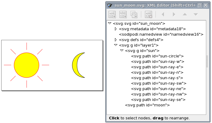
The image features a sun and a moon. The sun consists of a circle and several
lines. They are grouped together, using the
Group
command from
Inkscape’s
Object
menu. The group can also be seen in the XML
representation, as an svg:g element, with the actual shapes (paths in this
case) as children. We assigned the sun id to the svg:g element, as it
represents the entire sun. For clarity we gave the sub-elements ids as well,
although that was not necessary, as we won’t directly reference them in the
CIF/SVG declarations.
The following CIF specification models the sun/moon example:
svgfile "sun_moon.svg";
automaton sun_moon:
cont t der 1.0;
location Day:
initial;
edge when t >= 12.0 do t := 0.0 goto Night;
location Night:
edge when t >= 12.0 do t := 0.0 goto Day;
svgout id "sun" attr "visibility"
value if Day: "visible" else "hidden" end;
svgout id "moon" attr "visibility"
value switch self:
case Day: "hidden"
case Night: "visible"
end;
endInitially, it is day (location Day). It is day for 12 hours, after which it
becomes night (location Night). After 12 hours, it becomes day again, etc.
There is one mapping to control the visibility of the sun, and one to control
the visibility of the moon. Changing the visibility of the svg:g group
element with id sun influences the visibility of all its children. This
saves us from having to control the visibility of all the individual shapes
that together represent the sun.
Both mappings map the current location of automaton sun_moon to either
"visible" or "hidden", although they do it in a different methods. The
mapping for the sun uses an if expression, which is shorter in syntax, and
especially suited for automata with only two locations. The mapping for the
moon uses a switch expression over self, which is a way to refer to
automaton sun_moon, from inside that automaton itself. The cases list all
the possible locations, and map them to the corresponding visibility values.
The switch method is a bit more explicit, and becomes more elegant as the
automaton has more locations.
The first part of this example shows a person walking on a floor, and features:
-
Grouping of SVG objects.
-
The position of grouped objects in SVG.
-
Changing the position of grouped objects using an output mapping.
-
Using the
scalestandard library function. -
Using text formatting.
The second part of this example shows a person walking around in a room, and features:
-
Using multiple values in an output mapping.
-
Using multiple format specifiers in a format pattern.
The following SVG image is used for the example of a person walking on a floor:
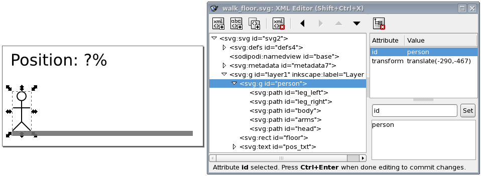
The image features a floor (gray bar), a person, and a text label. The
person consists of some lines and a circle. These shapes are grouped together,
using the
Group
command from Inkscape’s
Object
menu.
The group can also be seen in the XML representation, as an svg:g element,
with the actual shapes (paths in this case) as children. We assigned the
person id to the svg:g element, as it represents the entire person. For
clarity we gave the sub-elements ids as well, although that was not necessary,
as we won’t directly reference them in the CIF/SVG declarations.
Note that we moved the person as a whole, to the start of the floor. Since
svg:g elements don’t have an x and y attribute in SVG, Inkscape
applies a translation to move the group. This is reflected in the XML as a
transform attribute, with the translate(-290,-467) value. This
indicates that the person was moved 290 pixels to the left, and 467 pixels to
the top (as SVG has its origin in the upper left corner of the canvas).
To get rid of this, once the person is at the correct initial position, we
can ungroup the person group (
Ungroup
command from Inkscape’s
Object
menu), and regroup it. By ungrouping the group, the
transformation is pushed to the individual elements of the group. The regroup
simply adds a new group around the elements, without a translation
transformation. The new group is given an automatically generated name, so we
need to rename it to person. This ungroup/group trick is often very useful.
After this trick, the image looks as follows:
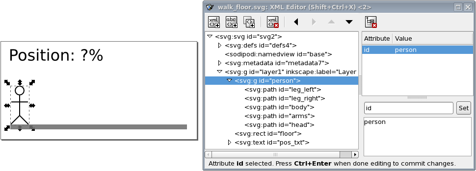
The text label is to be used to show the position of the person, as a
percentage. The left position is represented as 0%, and the right position is
represented as 100%. The id of the text label is pos_txt.
The following CIF specification models a person walking on a floor:
// Behavior.
automaton person:
cont pos = 0.0;
location forward:
initial;
equation pos' = 1.0;
edge when pos >= 5.0 goto backward;
location backward:
equation pos' = -1.0;
edge when pos <= 0.0 goto forward;
end
// Visualization.
svgfile "walk_floor.svg";
// width of the floor - width of the person = movement
// 180px - 19px = 161px
svgout id "person" attr "transform"
value fmt("translate(%s,0)", scale(person.pos, 0, 5, 0, 161));
svgout id "pos_txt" text
value fmt("%.1f%%", scale(person.pos, 0, 5, 0, 100));A person starts at position (variable person.pos) zero (value 0.0), and
initially moves forward. After (s)he has reached position 5.0, the
movement is reversed. Once the person is back at the start position, the
movement repeats itself.
There are two mappings, one that controls the horizontal position of the
person, and another that controls the text of the text label.
As stated above, the values of variable person.pos are in the range
[0 .. 5]. As can be seen from the comments of the CIF model, the width of the
floor and person are 180 pixels and 19 pixels respectively. The person can
thus move 161 pixels to the right. The output interval of the scale
standard library function is thus [0 .. 161]. As the vertical position is
fixed, no vertical translation is required. The
format pattern
"translate(%s,0)" inserts the scaled value into the horizontal amount of
the translation. The formatted output updates the transform attribute,
making the person move horizontally.
The text of the text label with id pos_txt is updated using a second
mapping. The value of variable person.pos is once again scaled using the
scale standard library function. This time the output range is [0 .. 100],
to get a percentage. Format pattern "%.1f%%" uses a %.1f format
specifier to convert that percentage to a textual value, with a single digit
after the decimal point. After the value of the percentage, a percentage
character is included in escaped form (%%), to ensure it is not interpreted
as a format specifier.
The following SVG image is used for the example of a person walking around in a room:
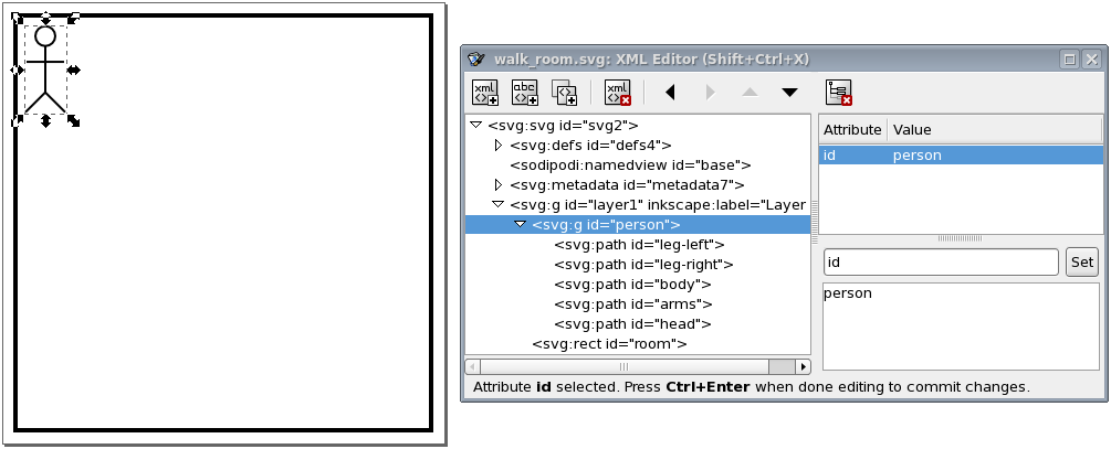
The image features a room (black rectangle) and a person. The person is the same group of elements as in the example of a person walking on a floor. The same group/ungroup trick is used here as well, to make sure the group has no translation transformation.
The following CIF specification models a person walking around in a room:
// Behavior.
automaton person:
cont x = 0.0;
cont y = 0.0;
location right:
initial;
equation x' = 1.0;
equation y' = 0.0;
edge when x >= 5.0 goto down;
location down:
equation x' = 0.0;
equation y' = 1.0;
edge when y >= 5.0 goto left;
location left:
equation x' = -1.0;
equation y' = 0.0;
edge when x <= 0.0 goto up;
location up:
equation x' = 0.0;
equation y' = -1.0;
edge when y <= 0.0 goto right;
end
// Visualization.
svgfile "walk_room.svg";
// width of the room - width of the person = horizontal movement
// 180px - 19px = 161px
//
// height of the room - height of the person = vertical movement
// 180px - 40x = 140px
svgout id "person" attr "transform"
value fmt("translate(%s,%s)", scale(person.x, 0, 5, 0, 161),
scale(person.y, 0, 5, 0, 140));A person starts at the top left position, and initially moves to the right.
Once (s)he reaches the right side, (s)he start to move down, followed by
a left and up movement. After the up movement, the person is once
again at the top left position, start another walk around the room, etc.
There is only one mapping, which controls both the horizontal and vertical
position of the person. The mapping is similar to the example of a person
walking on a floor, except that now both the horizontal and vertical movements
are included. The mapping uses two scaled values, one for the horizontal
movement, and one for the vertical movement. The format pattern includes both
values in the output. The first scaled value controls the horizontal movement,
while the second scaled value controls the vertical movement.
This example shows:
-
The use of literal values in output mappings.
-
How it is best to use simple solutions to solve visualization problems.
The following SVG image is used for this example:
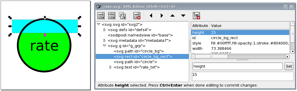
The SVG image visualizes a machine as a circle. The rate of the machine is visualized as the background of the circle. The higher the rate, the more the circle is filled.
Instead of working with complicated clippings or linear gradients, we use a
more simple solution here. The black circle has a transparent background
(fill attribute set to none). This is the SVG element with id
circle. Behind it is the same circle (id circle_bg), but without a
border (stroke attribute set to none), and with a green fill color.
Between those two circles, is a rectangle (id circle_bg_rect), that at the
top is aligned to the top of the circle. By changing the height of the circle,
we can now control what part of the green background circle is obscured by the
rectangle.
During the actual visualization, we’ll use a white fill color for the rectangle. Since the background is also white, this 'hides' the rectangle, and makes for a partial green background of the circle. Because a white rectangle can not be distinguished from the background, we used a cyan fill color for the rectangle. This makes that we can easily edit the rectangle, and see whether it has the correct initial position, size, etc.
The following CIF specification models the rate example:
// Behavior.
const real MARGIN = 0.01;
automaton machine:
cont rate der if rate < target_rate: 1.0
else -1.0
end;
disc real target_rate = 0.5;
disc dist real rate_sampler = uniform(0.0, 1.0);
location:
initial;
edge when rate - MARGIN <= target_rate and target_rate <= rate + MARGIN
do (target_rate, rate_sampler) := sample rate_sampler;
end
// Visualization.
svgfile "rate.svg";
svgout id "circle_bg_rect" attr "height"
value scale(machine.rate, 0, 1, 58, 0);
svgout id "circle_bg_rect" attr "fill" value "white";This rather artificial machine has a rate at which it produces. The rate
is a value in the interval [0 .. 1]. A target rate (variable target_rate)
is randomly chosen in the same interval. The rate is automatically adapted to
get closer to the target rate. As soon as the rate is close enough to the
target rate, a new target rate is randomly selected, using the
rate_sampler, which is a continuous uniform stochastic distribution.
The first mapping controls the height of the rectangle. The value of
variable machine.rate has a value in the interval [0 .. 1]. This interval
is mapped to the [58 .. 0] pixels interval. That is, if the rate is 0, the
height of the rectangle is 58 pixels, and it completely covers the background
of the circle. The circle then appears with a completely white background. If
the rate is 1, the height of the rectangle is 0, and a completely green
background is shown. For rates in between 0 and 1, the lower part of the
background of the circle is green, and the upper part is white.
The second mapping sets the fill color of the rectangle to white.
The following image shows an example of the visualization of a partial rate:

This example shows:
-
Basing the width of an object on the value of a clock in one location, and setting it to a fixed value in another location.
-
Changing the fill color of a rectangle based on the current location of an automaton.
-
Updating multiple attributes of an SVG element, using multiple output mappings.
-
Specifying colors in SVG.
-
Improving scalability by making use of the reuse of mappings.
The following SVG image is used for this example:

In the image, two machines are clearly visible. Each machine has a bar that
shows the progress of the machine. Looking at the
XML Editor
window, we can see the bar has a background (box), and a foreground (front)
rectangle. The width and fill color of the latter will be updated to
reflect the machine’s status.
The following CIF specification models the workstation example:
svgfile "workstation.svg";
event generate, transfer, exit;
m1: Machine(1, 1.0, generate, transfer);
m2: Machine(2, 2.5, transfer, exit);
automaton def Machine(alg int nr; alg real ptime; event start, done):
cont t der 1.0;
location idle:
initial;
edge start do t := 0.0 goto processing;
location processing:
edge when t >= ptime goto completed;
location completed:
edge done goto idle;
svgout id "m" + <string>nr + "_bar_front" attr "width"
value scale(if processing: t else ptime end, 0, ptime, 0, 130);
svgout id "m" + <string>nr + "_bar_front" attr "fill"
value if idle : "gray" else "dodgerblue" end;
endThe example models a workstation with two machines. The first machine has a
processing time of 1.0 time units and the second machine has a processing
time of 2.5 time units. Each machine gets products to start processing,
processes them, and sends them out as it is done. The first machine gets
its input from an infinite generator (event generate). The second machine
sends its finished products to an infinite exit buffer (event exit).
Products are transported from the first machine to the second machine via a
transport system (event transfer). Note that the Machine automaton
definition has three locations. In location idle it is waiting for a
product to enter the machine (event start). In location processing it
processes the product, which takes ptime time units. Finally, in location
completed it has completed processing the product, and waits until it can
send it as output. After that, the machine is back in the idle location,
where it waits for the next product.
Both machines (m1 and m2) are instantiations of the same automaton
definition (Machine). The definition/instantiation mechanism allows us to
specify the behavior of a machine only once, and still have multiple machines.
This reuse improves scalability, as well as maintainability. The reuse of the
behavior applies to the visualization as well. By declaring the output mappings
in the automaton definition, we get mappings for each instantiation of an
actual machine.
Since each machine has its own graphical representation in the SVG image, the
graphical elements for the different machines have different ids as well.
However, they only differ in the number that is used. For instance, there is
an m1_bar_front rectangle for the first machine, and an m2_bar_front
rectangle for the second machine. In order to make sure each machine gets the
correct mappings that apply to their own ids, we added an algebraic parameter
nr to the definition of Machine, that indicates to the machine which
machine it is. We can then use that nr to compute the id. For machine
m1, the Machine automaton definition is instantiated with value 1
for the nr parameter. The "m" + <string>nr + "_bar_front" id expression
then evaluates to "m1_bar_front", and m1_bar_front is used as the id
for the output mapping.
The first mapping updates the width of the m*_bar_front rectangles to show
the progress of the machines. If a machine is actually processing, the
value of clock t is used, as that clock indicates how much of the
processing has been completed.
When a machine is idle (and waiting for a product) or has completed
processing (but can not yet push the processed product out of the machine),
the progress is either nothing, or everything. In both cases, we choose the
full processing time (variable ptime) as the value. The reason to choose
this value for the idle location, becomes clear in the next output mapping.
The ptime value is chosen for the completed location to ensure that
the rectangle does not get wider than the box (rectangle m*_bar_back). If
we would have used the value of clock t in this location as well, then
since the value of the clock keeps increasing in that location, the value
becomes larger than ptime, and thus the progress bar would be partly
outside the box (rectangle m*_bar_back).
The value that is selected for this first mapping, is transformed using the
scale standard library function. The function is used to scale the
processing time interval [0 .. ptime] to the [0 .. 130] interval, which
represents the width of the rectangle in pixels. The upper bound of 130
pixels matches the width of the box (rectangle m*_bar_back).
The second mapping updates the fill color (foreground color) of the same
SVG element. In the idle location, the color is gray. Since we used the
full width in that location (value ptime in the [0 .. ptime] interval),
the entire box is then filled by a gray rectangle, indicating that the machine
is idle.
For the other locations, the fill color is set to dodgerblue. Since the
width in pixels is a value in the interval [0 .. 30], part of the box will be
blue, and part will be the background color of the box, which is white. In the
completed location, the full width is used as well, resulting in a
completely blue box, indicating that the machine has a completely processed
product, waiting to be released as output.
In the mappings, as described above, we used names to identify colors. SVG however, provides several ways to specify colors:
-
Named colors, such as
red,yellow,lightblueorburlywood. -
Decimal RGB (red-green-blue) colors, such as
rgb(255,0,0)forred, orrgb(255,255,0)foryellow. -
Hexadecimal RGB (red-green-blue) colors, such as
#f00or#ff0000forred, or#ff0or#ffff00foryellow. -
RGB (red-green-blue) colors in percentages, such as
rgb(100%,0%,0%)forred, orrgb(100%,100%,0%)foryellow.
Every color can be specified by one of the three RGB color variants. The colors that have a predefined color name, can be specified in four different ways.
This example shows:
The following SVG image is used for this example:
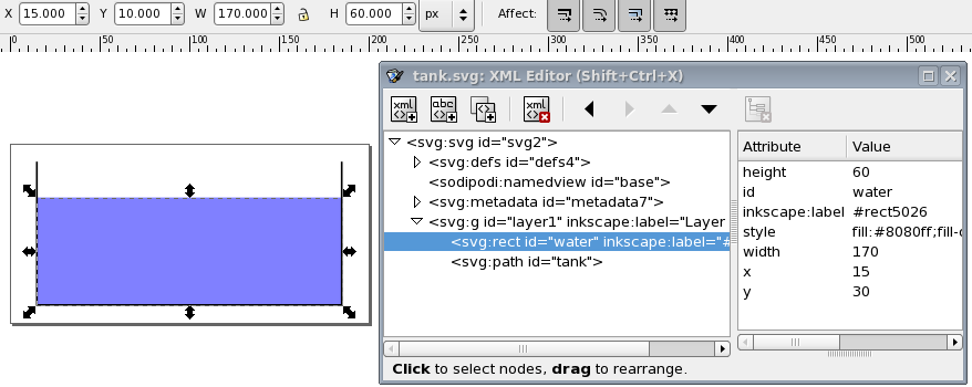
The image features a tank (black lines) and the water in the tank (blue
rectangle). The water rectangle is selected. At the top of the screenshot, you
see the object’s position as Inkscape represents it. It shows 15 for the
x position, and 10 for the y position. These values are relative to
the lower left corner of the canvas. In the
XML Editor
window, you
see the position as SVG represents it. It shows 15 for the x position
as well, but 30 for the y position. These values are relative to the
upper left corner of the canvas. Inkscape and SVG use different coordinate
systems, where the y-axis is reversed. The CIF/SVG declarations works on
SVG images, and thus uses the coordinate system of SVG.
The following CIF specification models the tank example:
// Behavior.
const real CAPACITY = 10.0;
const real MAX_LEVEL = 8.0;
const real INIT_LEVEL = 5.0;
const real MIN_LEVEL = 2.0;
automaton tank:
cont level = INIT_LEVEL;
location open:
initial;
equation level' = 1.0;
edge when level >= MAX_LEVEL goto closed;
location closed:
equation level' = -1.0;
edge when level <= MIN_LEVEL goto open;
end
// Visualization.
svgfile "tank.svg";
svgout id "water" attr "height" value scale(tank.level, 0, CAPACITY, 0, 80);In this specification, we have a tank filled with water. Initially, the
level (height) of the water is 5.0, and the valve is open. The
level linearly increases with a rate of 1.0 per time unit. Once the level
is MAX_LEVEL, we close the valve, and go to the closed location. Here
the level linearly decreases until we reach the minimum level (MIN_LEVEL),
after which we open the valve again. The level controller keeps the level
between the minimum and maximum allowed levels.
There is only one mapping, and it controls the height of the water
rectangle. The water level in the model stays between zero and CAPACITY, by
definition (as a higher level would overflow). This results in an input
interval of [0 .. CAPACITY]. The height of the tank in the SVG image is
80 pixels. The output interval thus becomes [0 .. 80].
When we simulate the tank example using the CIF specification and SVG image as specified above, we immediately observe a problem:

In SVG the origin is in the upper left corner of the canvas. Changing the height of an object results in the top of the object being fixed, and the bottom of the object being closer to or farther away from that top. What we want in this case, is to have the bottom of the object fixed, and the top of the object being closer to or farther away from the top, depending on the height of the object.
A naive solution would be to add a second output mapping, to correct the
vertical position (y attribute) of the water rectangle. This is a valid
solution, and it works. There is however a simpler and more elegant solution.
Consider the following, updated SVG image:
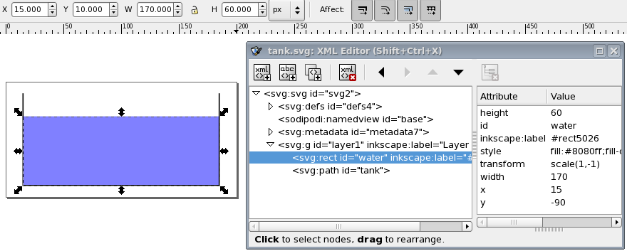
This SVG image is the same as the original SVG image for this example, but with
an inverted y-axis, for the water rectangle. The y-axis was
inverted by using the
Flip Vertical
command from Inkscape’s
Object
menu, while the water rectangle was selected. As can be
seen in the screenshot, Inkscape corrects for the applied transformation, and
still indicates the same x and y coordinates (at the top of the
screenshot). In SVG (and thus the
XML Editor
window), we see a new
transform attribute, scale(1,-1) as value, which represents the
inversion of the y-axis. Also, the bottom of the water (the inverted top of
the water) is now 90 pixels (the inverted -90 value of the y
attribute) from the top of the image. Using this vertical flip, we now fixated
the 'bottom' of the water, and we can thus change the height of the water
without having to correct its position. The mappings for this modified SVG
image are the same as the original mappings.
This example shows:
-
Scalability of CIF models and SVG visualizations.
-
The use of CIF/SVG copy declarations.
-
The use of CIF/SVG move declarations.
Consider the following CIF specification:
// Behavior.
automaton def Lamp():
event toggle;
disc bool on = false;
location:
initial;
edge toggle do on := not on;
end
lamp1: Lamp();
lamp2: Lamp();
// Visualization.
svgfile "lamps2.svg";
svgout id "lamp1" attr "fill" value if lamp1.on: "yellow" else "silver" end;
svgout id "lamp2" attr "fill" value if lamp2.on: "yellow" else "silver" end;
svgout id "lamp1" attr "stroke-width" value if lamp1.on: 5 else 2 end;
svgout id "lamp2" attr "stroke-width" value if lamp2.on: 5 else 2 end;This specification has two lamps, lamp1 and lamp2. Both lamps have
identical behavior, and therefore the behavior is only specified once, using
automaton definition Lamp. This definition is instantiated two times, once
for each of the lamps. A lamp is initially off, can go on, go off again, go on
again, etc. The following SVG image is used for this example:

The visualization shows the two lamps. The first lamp is off, and has a silver background color. The second lamp is on and has a yellow background color. The lamp that is off has a thin border and the lamp that is on has a thicker border. The CIF specification also contains four CIF/SVG output mappings, two for the background colors of the circles and two for the thickness of the borders (strokes) of the circles.
The use of the automaton definition allows us to add another lamp by simply adding the following line to the CIF specification:
lamp3: Lamp();This single line ensures that we have a third lamp, with the corresponding behavior. However, we also need to adapt the SVG image, by adding another circle, and we need to add two more output mappings to the CIF model. In this case, the additional amount of work is manageable. If however our lamp would have been represented in the image by many different graphical elements, adding another lamp would require copying all those graphical elements, and might also lead to adding many more output mappings per lamp.
Furthermore, if we were to decide to change the graphical representation of lamps from a circle to a square, we would have to change the graphical representation of each of the lamps in the image.
It should be clear that this approach does not scale very well. Ideally, we
would add another lamp by just adding another instantiation of the Lamp
definition as we did above, and automatically get another circle in the image,
and two more output mappings in the CIF model.
For the behavior of the lamp, we already had a scalable solution, by using the component definition/instantiation mechanism. That same mechanism can be used to make the image and mappings scalable. First, we’ll change the SVG image:

The second lamp has been removed from the image. We only keep one lamp, as a
sort of template for all the lamps. Since we want to use the same graphical
representation for all lamps, we only want to include it once in the SVG image.
This allows us to change the graphical representation of the template, to have
all the lamps change appearance at once. The lamp has been moved outside of the
visible part of the canvas, and its id has been changed from lamp1 to
lamp. The reason for these last two changes will become clear once we look
at the new CIF model, and especially the new output mappings:
svgfile "lamps3.svg";
automaton def Lamp(alg int nr):
// Behavior.
event toggle;
disc bool on = false;
location:
initial;
edge toggle do on := not on;
// Visualization.
svgcopy id "lamp" post <string>nr;
svgmove id "lamp" + <string>nr to 20 + (nr - 1) * 100, 20;
svgout id "lamp" + <string>nr attr "fill"
value if on: "yellow" else "silver" end;
svgout id "lamp" + <string>nr attr "stroke-width"
value if on: 5 else 2 end;
end
lamp1: Lamp(1);
lamp2: Lamp(2);
lamp3: Lamp(3);The first change is that the Lamp automaton definition now has a nr
parameter, that indicates which lamp it is. Each lamp is given a different
number when instantiated. This allows the lamp automata to know their own
identity, and use that for the SVG visualization.
We also put the CIF/SVG declarations for the visualization inside the automaton definition. By doing this, we ensure that each instantiation (each lamp) gets their own version of these declarations.
The CIF/SVG declarations have changed as well. A
CIF/SVG copy declaration has been added. The copy
declaration states that the SVG element with id lamp (the circle) should
be copied. It also states that the copy should be postfixed with
<string>nr. That is, for automaton lamp1, the value of the nr
parameter is 1, and the id is thus postfixed with "1". In other words,
circle lamp is copied, and the copy is given name lamp1 (composed
from lamp and 1). For lamp2, the id of the copied circle is
lamp2, etc. For each of the lamps, the copy gets a different name, that is
unique within the SVG image. This single copy declaration takes care of the
scalability of the SVG image, by ensuring we have exactly as many circles as we
have lamps (not counting the template circle lamp).
The copies of the template circle all get exactly the same attributes as the
template (except for their id attribute). As such, they are all positioned
outside the visible part of the canvas. The easiest way to put them at the
correct positions, is to use a
CIF/SVG move declaration, which
is also new compared to the previous CIF model. The move declarations use the
ids of the copied circles, so that each move declaration moves the circle for
that specific lamp. They are all moved to 20 pixels from the top of the canvas,
and '20 + (nr - 1) * 100' pixels from the left side of the canvas. So, the
first lamp (nr 1) is moved to (20, 20), the second lamp (nr 2) is moved
to (120, 20), and the third lamp (nr 3) is moved to (220, 20). This single
move declaration takes care of the scalability of the positions of the lamps,
by ensuring we have exactly as many movements as we have lamps. By using the
nr parameter, each lamp can easily be moved to their own unique position.
The output mappings for the background color of the circles and thickness of
the borders of the circles, are very similar to the output mappings of the
first version of the CIF model, though there are a few changes. The mappings
use the same method as the move declaration, to construct the ids. Since the
mappings are now defined within the automaton definition, they can directly
refer to the on variable. This ensures that for each different lamp, the
mappings refer to the on variable of that specific lamp. We now have only
one output mapping for the background color, and also only one output mapping
for the thickness of the border.
By putting the CIF/SVG declarations inside the automaton definition, and by
using the copy and move declarations, we now have a scalable solution. We only
have one lamp in our SVG image, only one behavioral specification in the CIF
model, and only one output mapping per attribute that we want to couple. No
matter how many instantiations of the Lamp automaton definition we add, we
don’t have to manually change the SVG image or the visualization coupling.
For completeness, take a look at this CIF model after the elimination of component definition/instantiation, the elimination of algebraic variables, and the simplification of values.
automaton lamp1:
event toggle;
disc bool on = false;
svgcopy id "lamp" post "1";
svgmove id "lamp1" to 20, 20;
svgout id "lamp1" attr "fill" value if on: "yellow" else "silver" end;
svgout id "lamp1" attr "stroke-width" value if on: 5 else 2 end;
location:
initial;
edge toggle do on := not on;
end
automaton lamp2:
event toggle;
disc bool on = false;
svgcopy id "lamp" post "2";
svgmove id "lamp2" to 120, 20;
svgout id "lamp2" attr "fill" value if on: "yellow" else "silver" end;
svgout id "lamp2" attr "stroke-width" value if on: 5 else 2 end;
location:
initial;
edge toggle do on := not on;
end
automaton lamp3:
event toggle;
disc bool on = false;
svgcopy id "lamp" post "3";
svgmove id "lamp3" to 220, 20;
svgout id "lamp3" attr "fill" value if on: "yellow" else "silver" end;
svgout id "lamp3" attr "stroke-width" value if on: 5 else 2 end;
location:
initial;
edge toggle do on := not on;
end
svgfile "lamps3.svg";This example shows:
-
Improving hierarchical scalability by making use of the reuse of mappings.
-
Improving hierarchical scalability by making copies of copied elements.
It is assumed the reader is already familiar with the workstation example.
The following SVG image is used for this example:

The SVG image contains a single template for a buffer (large rectangle), with one product (small rectangle). The template is moved outside of the canvas to ensure the template itself is not shown.
The SVG file has the following XML content:
<?xml version="1.0" encoding="UTF-8" standalone="no"?>
<svg xmlns="http://www.w3.org/2000/svg"
xmlns:svg="http://www.w3.org/2000/svg"
width="220" height="70" id="root" version="1.1">
<g id="buffer">
<rect width="100" height="50" x="-120" y="10" id="background" style="fill:#ff0000"/>
<rect width="10" height="30" x="-110" y="20" id="product" style="fill:#8b0000;visibility:hidden;"/>
</g>
</svg>We’ll use CIF to turn this into two buffers with three products each, in a scalable manner. That is, to add a single buffer, we only need one more instantiation, and also to put an additional product in each buffer, we also only need one more instantiation.
The following CIF specification models the buffers/products example:
svgfile "buffers_products.svg";
buffer0: Buffer(0);
buffer1: Buffer(1);
group def Buffer(alg int nr):
svgcopy id "buffer" post <string>nr;
svgmove id "buffer" + <string>nr to 10 + nr * 110, 10;
product0: Product(nr, 0);
product1: Product(nr, 1);
product2: Product(nr, 2);
end
group def Product(alg int bufferNr, productNr):
svgcopy id "product" + <string>bufferNr post "_" + <string>productNr;
svgout id fmt("product%d_%d", bufferNr, productNr)
attr "transform"
value fmt("translate(%d,0)", productNr * 20);
svgout id fmt("product%d_%d", bufferNr, productNr)
attr "visibility"
value "visible";
endTwo buffers are present (buffer0 and buffer1). Both are instances of
the Buffer definition, and are provided with their own identity (parameter
nr). For each buffer, the buffer element of the image is copied, and
the copy is given a unique number. For instance, for instantiation buffer0,
nr is 0, and thus buffer is copied to buffer0, background
is copied to background0 and product is copied to product0.
Each buffer is also moved. The first buffer (nr 0) gets moved to
position (10, 10), while the second (nr 1) gets moved to position
(120, 10).
Each buffer contains three products, as the Product definition is
instantiated three times. The number of the buffer is passed along, as is a
unique product number. For the copy of the products, the copy of the product
in the copied buffer is copied, and given a unique name using the product
number. For buffer0, the copy of the product was already named
product0. This already copied element is copied another three times, to
product0_0 (by the copy declaration in CIF group buffer0.product0),
product0_1 (by the copy declaration in CIF group buffer0.product1),
and product0_2 (by the copy declaration in CIF group buffer0.product2).
Similarly, three copies are made for buffer1.
Unlike the buffers, which are moved to an absolute position using an
svgmove, the products are moved relatively, using an svgout for their
transform attribute. The first product (product0_0) is not moved, the
second product (product0_1) is moved 20 pixels, etc.
The buffer template was put outside of the canvas to show only the copies and
not the template. For the products, which are contained in the buffers, this
trick is not possible. So, instead the visibility of the template
product was set to hidden in the original SVG image. To show the actual
(copied) products, an svgout is used to set the visibility attribute
to visible. The template product is not changed, so it remains hidden.
The result of all this hierarchical 2-level structure is the following SVG image:

Trajectory data output
The trajectory data (values of the variables as time progresses), calculated by the ode solver, can be written to a file, using the trajectory data output component.
Enable the Trajectory data option (Output: Trajectory data category) to enable writing the trajectory data to a file.
By default, the file to which to write the trajectory data, is the name of the
input specification file, with .trajdata added to it. Using the
Trajectory data file
option (Output: Trajectory data
category), a different file can be specified. The value of the option is the
absolute or relative local file system path to use for the trajectory data
file.
Variable time is always included in the trajectory data file. The following
additional variables (officially 'state objects') are included by default:
-
The state variables, which includes the discrete variables and the continuous variables.
-
The derivatives of the continuous variables. This does not include the derivative of variable
time. -
The algebraic variables.
Only variables of type bool, int (with or without ranges), or real
are included.
Using the Trajectory data filters option (Output: Trajectory data category), the state objects can be filtered. The Trajectory data filters option only has effect if trajectory data output is enabled, using the Trajectory data option.
As value for the option, comma separated filters should be supplied. Each
filter specifies one or more state objects. The absolute names of the objects
are used. That is, for an automaton a, with a variable x, the absolute
name of the variable object is a.x. If CIF textual syntax keyword are
used as names for events (such as plant), then they must be escaped in
.cif files ($plant). For filters however, all escape characters ($)
in the names are ignored. The * character can be used as wildcard, to
indicate zero or more characters. If a filter doesn’t match any of the state
objects of the CIF model (after filtering them for supported types etc), a
warning is printed to the console. A warning is also printed if the entire
state is filtered out.
By default, filters include matching state objects. Filters may however be
preceded by a - character, turning them into exclusion filters, which
exclude matching states objects rather than including them. Filters are
processed in the order they are specified, allowing for alternating additions
and removals. If a filter does not result in the addition/removal of any state
objects to/from the filter result, a warning is printed to the console.
As an example, option value a.*,-a.b*,a.bc* consists of three filters:
a.*, -a.b*, and a.bc*. The first filter indicates that state
objects whose absolute names start with a. are to be included. The second
filter indicates that from those matching state objects, the state objects
whose absolute names start with a.b* are to be excluded. To that result,
the third filter adds those state objects whose absolute names start with
a.bc*. For instance, if a specification contains state objects time,
a.a, a.b a.bb, a.bc, a.b.c, a.bc, a.bcc, and
a.bcd, the result of the three filters is that the following state objects
are displayed: a.a, a.bc, a.bc, a.bcc, and a.bcd.
The default option value (filter) is *.
The variables are sorted alphabetically, based on their absolute names. The
only exception is variable time, which is always listed first.
For variables with a boolean type, value false is represented by 0, and
value true is represented by 1.
For each time transition, the trajectories of the variables are printed to the
trajectory data file. The first line is a comment, and contains the names of
the variables. Each of the subsequent lines contain the values of the variables
for a specific value of variable time. The exact times for which the
values are printed to the trajectory data file, is determined by the
ODE solver integrator, and can be
influenced using the integration options,
as well as the fixed output step size option.
An example of a trajectory data file, for a single time transition:
# time controller.n tank.V tank.V' tank.Qi tank.Qo
0.0 0 10.0 -3.1622776601683795 0.0 3.1622776601683795
0.08763429266802605 0 9.7247959763441 -3.1184605138343664 0.0 3.1184605138343664
0.587634292668026 0 8.228065719426915 -2.868460513834366 0.0 2.868460513834366
1.087634292668026 0 6.8563354625097315 -2.618460513834366 0.0 2.618460513834366
1.587634292668026 0 5.609605205592543 -2.3684605138343646 0.0 2.3684605138343646
2.0876342926680262 0 4.487874948675351 -2.1184605138343624 0.0 2.1184605138343624
2.5876342926680262 0 3.491144691758149 -1.8684605138343569 0.0 1.8684605138343569
3.0876342926680262 0 2.619414434840913 -1.618460513834339 0.0 1.618460513834339
3.496128195593086 0 1.9999999999999958 -1.4142135623730936 0.0 1.4142135623730936To make the output in the trajectory data file easier to read, the output can be prettified. If prettifying is enabled, then after the simulation ends, the trajectory data file is read, prettified, and rewritten. A fixed width is then used for each column (each variable), with a fixed column separation. After prettification, the above trajectory data file looks like this:
# time controller.n tank.V tank.V' tank.Qi tank.Qo
0.0 0 10.0 -3.1622776601683795 0.0 3.1622776601683795
0.08763429266802605 0 9.7247959763441 -3.1184605138343664 0.0 3.1184605138343664
0.587634292668026 0 8.228065719426915 -2.868460513834366 0.0 2.868460513834366
1.087634292668026 0 6.8563354625097315 -2.618460513834366 0.0 2.618460513834366
1.587634292668026 0 5.609605205592543 -2.3684605138343646 0.0 2.3684605138343646
2.0876342926680262 0 4.487874948675351 -2.1184605138343624 0.0 2.1184605138343624
2.5876342926680262 0 3.491144691758149 -1.8684605138343569 0.0 1.8684605138343569
3.0876342926680262 0 2.619414434840913 -1.618460513834339 0.0 1.618460513834339
3.496128195593086 0 1.9999999999999958 -1.4142135623730936 0.0 1.4142135623730936By default, the trajectory data output is prettified using a column separation of three spaces. This can be changed using the Trajectory data separation amount option (Output: Trajectory data category). Using this option, prettification can be disabled, or a different number of spaces can be used between the columns.
It is possible to go back in time, by undoing one or more transitions, or by resetting the simulation. However, once a time transition is taken, trajectory data is written to the output file. The simulator does not remove data for time points that are then suddenly in the future. If simulation continues after the undo or reset, new data may be written at the end of the trajectory, for the same time points that were already present earlier in the data file. As such, the data contained in the trajectory data file, may no longer be useful after an undo or reset, if simulation continues afterwards.
Plot visualizer
For models with variables, especially continuous ones, it may be useful to be
able to observe how their values change, as time progresses during simulation.
The plot visualizer can be used for that exact purpose. The plot visualizer
can create graphical plots, where the x-axis represents the values of variable
time, and the y-axis represents values of the variables being plotted. Here
is an example screenshot of the visualizer:

Plot visualization is disabled by default. It can be enabled using the Plot visualization option (Output: Plot visualization category).
The plot visualizer can plot the values of the following variables (officially 'state objects'):
-
The state variables, which includes the discrete variables and the continuous variables.
-
The derivatives of the continuous variables. This does not include the derivative of variable
time. -
The algebraic variables.
Only variables of type bool, int (with or without ranges), or real
can be plotted. For variables with a boolean type, value false is
represented by 0, and value true is represented by 1.
By default, if plot visualization is enabled, all variables (officially
'state objects') that can be plotted are plotted. The one exception is variable
time, which is excluded by default, as it already represents the x-axis.
That is, variables are plotted against time. Using the
Plot visualization filters
option
(Output: Plot visualization
category), the state objects can
be filtered. The
Plot visualization filters
option only has effect
if plot visualization is enabled, using the
Plot visualization
option.
As value for the option, comma separated filters should be supplied. Each
filter specifies one or more state objects. The absolute names of the objects
are used. That is, for an automaton a, with a variable x, the absolute
name of the variable object is a.x. If CIF textual syntax keyword are
used as names for events (such as plant), then they must be escaped in
.cif files ($plant). For filters however, all escape characters ($)
in the names are ignored. The * character can be used as wildcard, to
indicate zero or more characters. If a filter doesn’t match any of the state
objects of the CIF model, a warning is printed to the console. A warning is
also printed if the entire state is filtered out.
By default, filters include matching state objects. Filters may however be
preceded by a - character, turning them into exclusion filters, which
exclude matching states objects rather than including them. Filters are
processed in the order they are specified, allowing for alternating additions
and removals. If a filter does not result in the addition/removal of any state
objects to/from the filter result, a warning is printed to the console.
As an example, option value a.*,-a.b*,a.bc* consists of three filters:
a.*, -a.b*, and a.bc*. The first filter indicates that state
objects whose absolute names start with a. are to be included. The second
filter indicates that from those matching state objects, the state objects
whose absolute names start with a.b* are to be excluded. To that result,
the third filter adds those state objects whose absolute names start with
a.bc*. For instance, if a specification contains state objects time,
a.a, a.b a.bb, a.bc, a.b.c, a.bc, a.bcc, and
a.bcd, the result of the three filters is that the following state objects
are displayed: a.a, a.bc, a.bc, a.bcc, and a.bcd.
The default option value (filter) is *,-time.
By default, only one visualizer is shown. However, using the Plot visualization filters option (Output: Plot visualization category), it is possible to specify that multiple visualizers should be used. The option allows for filtering of the state objects, as described above. However, such filters can be separated by semicolons, to specify the filters per visualizer.
As an example, consider option value time,a.x;b.y. This results in two
plot visualizers. The first one displays state objects time and a.x,
while the second one displays state object b.y.
There are two plot visualization modes:
-
Live plotting. In this mode, the plots are shown at the start of the simulation, and are continuously updated as new data becomes available during simulation.
-
Postponed plotting. In this mode, the plots are shown after the simulation has ended.
Which plot visualization mode to use, can be configured using the Plot visualization mode option (Output: Plot visualization category). Using that option it is possible to explicitly choose one of the modes. By default, an automatic mode is used, which chooses between live and postponed mode, as follows:
| Input mode vs real-time simulation | Real-time enabled | Real-time disabled |
|---|---|---|
Interactive console input mode (pure interactive) |
live |
live |
live |
postponed |
|
Interactive GUI input mode (pure interactive) |
live |
live |
live |
postponed |
|
live |
postponed |
|
live |
postponed |
|
live |
postponed |
When doing a non real-time simulation, using a non-interactive input mode leads to as fast as possible simulation, where a lot of data points are calculated in a short amount of time. If live plotting mode is then enabled, this floods the visualizer with so much data that it can’t keep up. The effect is a non-responsive user interface. While the automatic default can thus be overridden using the option, it is generally not recommended.
For simulations that span longer periods of (model) time, there may be too much data to display, for the limited width of the time axis (x-axis). To keep the plot useful, the range of time values to display on the x-axis can be configured using the Plot visualization range option (Output: Plot visualization category).
By default, only the 50 most recent time units are displayed. That is, if
the current model time is 120, then the plot only shows the values of the
variables from time 70 to time 120. Using the option, the length of the
range can configured to any other positive value. The option can also be used
to set the range to infinite, to display the values of the variables during
the entire simulation, from time 0 to the current model time.
For long running simulations, with lots variables, using an infinite range can lead to large numbers of data points, which can have a significant effect on performance. This applies especially for live plotting mode.
This section describes which data points are visualized. For most users, this will be of little interest, as it essentially works as you would expect.
The plot visualizer adds data points (a time value and a value of a
variable at that time) for all variables, for the following
states:
-
The initial state of the simulation.
-
The start state of every time transition.
-
Intermediate states of time transitions, only if real-time simulation is enabled.
-
Trajectory data points of time transitions, only if real-time simulation is disabled.
-
The end state of every time transition.
For real-time simulation, the amount of model time between two intermediate states is the model time delta, and can be influenced using the frame rate and simulation speed.
For non real-time simulation, the trajectory data points are determined by the ODE solver integrator, and can be influenced using the integration options, as well as the fixed output step size option.
The plot visualizer can be used for simple plotting. It can be customized a bit through options, as described above. However, the level of customization is somewhat limited. For instance, the appearance can not be customized. This is intentional.
If further customization is required, use the trajectory data output component instead. It allows saving the data to a file, for further processing with external tools, such as R.
Such post processing is then performed after the simulation has ended. A benefit of the plot visualizer, is that it allows live plotting mode, without the need of post processing, and which can be enabled with little effort. The plot visualizer is meant to be used only to get a basic understanding of how values of variables change as time progresses.
The plot visualizer can export the currently visible plot to several different image formats. To export the image, first make sure that the plot visualizer has the focus. Then select to open the Save plot as dialog. Alternatively, right click the plot itself, and choose Save As… from the popup menu, to open the Save plot as dialog. In the dialog, specify the file name of the exported image. Click OK to confirm and continue.
A second dialog appears, in which the size of the exported image can be
specified. By default, the current size of the visualizer is used. A custom
size can be entered. The width and height need to specified in pixels,
separated by a x character. For instance, for a width of 640 pixels and
a height of 480 pixels, enter 640x480 into the dialog. Click OK to
confirm and to actually export the image.
The following raster image formats are supported:
-
Portable Network Graphics (
*.png) -
JPEG (
*.jpg) -
Graphics Interchange Format (
*.gif)
The image format that is used to export the image, is derived from the file extension that is used. For each of the supported file formats, the allowed file names (with file extensions) are indicated above (between parentheses).
After the image is exported, the workspace is refreshed to show that new image file, if the image was saved in a project that is visible in the 'Project Explorer' tab or 'Package Explorer' tab.
In order for the export to succeed, data points must be available for at least two time values.
It is possible to go back in time, by undoing one or more transitions, or by resetting the simulation.
If one or more transitions are undone, data for all time points that are then suddenly in the future, are removed. More precisely, all data for time points added for time transitions that have been undone, are removed.
If the simulation is reset, the entire plot is cleared.
State visualizer
The normal console output, which may include the state of the specification, is printed to the console. The entire state is then printed as a single line of text, which can be hard to read as the specification grows, and the state contains more and more variables. The state visualizer can be used as an alternative. It shows the same information, but in a table in a separate window. Here is an example screenshot of the visualizer:
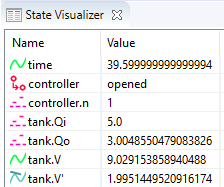
Unlike SVG visualization, which requires that the user makes an image of the system and couples the image to the specification, the state visualizer can be used directly, without any additional effort. All that is required to use it, is to enable it. The state visualizer is disabled by default, and can be enabled using the State visualization option (Output: State visualization category).
The state visualizer shows all the discrete, continuous, and algebraic
variables of the specification, as well as their values. It also shows the
derivatives of the continuous variables, and their values. This includes
variable time, but not its derivative. It also shows the automata, with
their current locations. The variables and automata are listed in alphabetical
order, except for variable time, which is always shown at the top.
The icons on the left indicate the kind of object that is shown in a particular row of the table:
-
 An automaton, with its current location.
 -
 A discrete variable, with its current value.
 -
 A continuous variable (includes variable
 time), with its current value. -
 A derivative of a continuous variable (excludes variable
time), with its current value. -
 An algebraic variable, with its current value.
The values are updated for the initial state, states reached after transitions (event transitions and time transitions), as well as for frames.
By default, all state objects are displayed by the state visualizer. Using the State visualization filters option (Output: State visualization category), the state objects can be filtered. The State visualization filters option only has effect if state visualization is enabled, using the State visualization option.
As value for the option, comma separated filters should be supplied. Each
filter specifies one or more state objects. The absolute names of the objects
are used. That is, for an automaton a, with a variable x, the absolute
name of the variable object is a.x. If CIF textual syntax keyword are
used as names for events (such as plant), then they must be escaped in
.cif files ($plant). For filters however, all escape characters ($)
in the names are ignored. The * character can be used as wildcard, to
indicate zero or more characters. If a filter doesn’t match any of the state
objects of the CIF model, a warning is printed to the console. A warning is
also printed if the entire state is filtered out.
By default, filters include matching state objects. Filters may however be
preceded by a - character, turning them into exclusion filters, which
exclude matching states objects rather than including them. Filters are
processed in the order they are specified, allowing for alternating additions
and removals. If a filter does not result in the addition/removal of any state
objects to/from the filter result, a warning is printed to the console.
As an example, option value a.*,-a.b*,a.bc* consists of three filters:
a.*, -a.b*, and a.bc*. The first filter indicates that state
objects whose absolute names start with a. are to be included. The second
filter indicates that from those matching state objects, the state objects
whose absolute names start with a.b* are to be excluded. To that result,
the third filter adds those state objects whose absolute names start with
a.bc*. For instance, if a specification contains state objects time,
a.a, a.b a.bb, a.bc, a.b.c, a.bc, a.bcc, and
a.bcd, the result of the three filters is that the following state objects
are displayed: a.a, a.bc, a.bc, a.bcc, and a.bcd.
The default option value (filter) is *.
By default, only one visualizer is shown. However, using the State visualization filters option (Output: State visualization category), it is possible to specify that multiple visualizers should be used. The option allows for filtering of the state objects, as described above. However, such filters can be separated by semicolons, to specify the filters per visualizer.
As an example, consider option value time,a.x;b.y. This results in two
state visualizers. The first one displays state objects time and a.x,
while the second one displays state object b.y.
Real-time simulation
The CIF simulator allows for a form of real-time simulation. By enabling
real-time simulation, the simulator interprets the model time (the value of
variable time) in seconds. The simulator attempts to ensure that the actual
simulation time is equal to the model time. This feature is very useful for
visualizers, which then visualize their output at a steady rate. Without
real-time simulation, the rate at which such visualizers would visualize their
output, would primarily be determined by the amount of time it takes for the
simulator to compute the output, leading to abrupt slow downs and sudden speed
increases.
If real-time simulation is disabled, visualizations are only updated for the states that are reached. That is, the visualizations are updated for the initial state, and each new state that is reached after taking a transition. The visual representations of the visualizations resulting from these states are called frames.
As time progresses, the values of continuous variables (and algebraic variables for which the value is directly or indirectly derived from a continuous variable, etc) change. If the visualization is only updated before and after time transitions, as is done when real-time simulation is disabled, this leads to 'jumps' in the visualization. For real-time simulation, the simulator calculates states that are evenly spaced over time. This ensures that we get regular updates of the visualizations, as time progresses, and the visualizations thus become 'smooth' or 'fluent'. If enough states are visualized per second, a visualization essentially becomes a movie.
The states that result from transitions are always calculated. For real-time simulation, the simulator calculates additional states for the purpose of visualization, as mentioned above. These additional states are called intermediate states, and the corresponding visual representations of the visualizations to which they lead are called intermediate frames.
For real-time simulation, the simulator thus uses intermediate frames that are evenly spaced over time, for smooth visualizations. A consequence of this, is that state changes between those intermediate frames are lost. If the effect is still visible in the next intermediate state, this is not a problem. If however the effect is temporary, and does not last until the next intermediate state, the effect is thus not visualized.
For real-time simulation combined with an interactive input mode, the simulator uses both the state frames and the intermediate frames. This ensures that at the moment an interactive choice has to be made about which transition to take, the visualization reflects the current state of the system. Semi-automatic mode is not taken into account.
Using the Frame rate option (Output category), it is possible to specify how often per second of real time, visualizations should be updated. A higher frame rate leads to more updates per second, and thus to a more fluent visualization. However, since a higher frame rate also leads to more frequent updates, the amount of CPU power it takes to perform these updates increases as well. If the computer can not update the visualization in time for the next update to take place, the visualization may start to 'stutter'.
The frame rate will thus always be a compromise between fluency and performance. Choosing an appropriate frame rate depends not only on the complexity of the specification being simulated and the visualization that is being shown, but also on the computer on which the simulation is run. Furthermore, it may depend on the other tasks the computer is performing while the simulation is being run.
Frame rates are always positive, and may be fractional. For instance, a frame
rate of 7.5 is valid, and will update the visualization 7.5 times per
second.
A low frame rate (typically less than 10 frames per second) can have a devastating effect on the responsiveness of SVG input. Similarly, it can hinder termination of the simulation, as the red Terminate button has no effect between intermediate frames. That is, the effect of clicking the button is postponed until the next frame, or until the time transition ends.
If real-time simulation is enabled, the simulator by default interprets the
model time (the value of variable time) in seconds. However, this can be
changed using the
Simulation speed
option (Output
category). This option specifies a scaling factor. A scaling factor of 1.0
interprets model time as seconds, 2.0 is twice as fast (1 unit of model
time takes 0.5 seconds), etc. The simulation speed must always be positive,
and may be fractional. For instance, a simulation speed of 0.5 is valid,
and will interpret model time as twice as slow (1 unit of model time takes 2
seconds).
By default, real-time simulation is disabled, and the simulator will try to
simulate as fast as possible (infinite speed, taking time transitions takes no
time). By setting a frame rate and/or a simulation speed, real-time simulation
can be enabled. If only one of the options is specified, the other gets a
default value. The default frame rate for real-time simulation is 20.0
frames per second. The default simulation speed is 1.0.
Enabling real-time simulation requires a real-time output component (visualizer). Currently, the following real-time output components are available:
If real-time simulation is enabled without using a real-time output component, simulation can’t be started. Closing the visualizer of a real-time simulation during the simulation, if it is the last remaining real-time output component, leads to the simulation being stopped.
All real-time output components can also be used when real-time simulation is disabled, but obviously without any real-time effects.
The simulation speed does not influence the frame rate. That is, both options
can be specified orthogonally. The two options together however, do influence
the model time delta, the amount of model time between two consecutive updates
of the visualizations, i.e. the amount of model time between two consecutive
intermediate frames. The model time delta is calculated using the following
formula (where r is the frame rate, and s is the simulation speed):
1 / (r / s). Doubling the frame rate results in half the model time
delta, while doubling the simulation speed results in double the model time
delta.
If the model time delta becomes to big, this may lead to 'jumps' in the visualization. In such cases, increasing the frame rate, or reducing the simulation speed causes a smaller model time delta, leading to a more fluent visualization.
The model time delta (and thus the frame rate and simulation speed) also affects the ODE solver fixed output step size.
Test mode disables all real-time delays of the real-time simulation mode, but still updates the visualizations for the intermediate frames. With test mode enabled, it is also allowed to perform a real-time simulation without real-time output component.
Simulation advanced topics
Simulator options
The CIF simulator can be configured via various options. The available options are listed below, per category.
General
-
Help: Prints the help text of the application to the console.
-
License: Prints the license text of the application to the console.
-
Developer mode: Option to control whether exceptional situations return limited and user-friendly information (the default), or extended developer oriented information. This option is primarily intended for the developers of the CIF simulator, and should not be used by end users.
Simulation
-
CIF specification: The absolute or relative local file system path to the CIF specification (
.ciffile) to simulate. May also be a compiled code file (.cifcodefile).
Compiler
Input
Output
Output: SVG visualization
Output: Trajectory data
Output: Plot visualization
Output: State visualization
ODE solver
ODE solver: ODE integrator
ODE solver: ODE root finder
Simulation performance
General performance information about Java or Eclipse typically applies to the CIF simulator as well. This page provides additional information specific to the CIF simulator.
Closing the simulator
Closing the simulator ensures that all its resources are freed, and become available for other applications. The CIF simulator however, may ask you to press ENTER to confirm termination of the simulator. If asked, as long as you haven’t pressed ENTER yet, the status of the console will still show it’s running, and the application can’t release its resources.
Slow starting of the simulator
If simulation is slow to start, you can try a different Java compiler. You can also try to compile the model once, reducing the start time of the simulator for repeated simulations.
Slow termination of the simulator
If termination of the simulator is slow, this may be related to the trajectory data output component. If its prettifying option is enabled, it will read the trajectory data file after the simulation terminates, and write the whole file again in a prettier from. This may take some time, especially on slow remote/network file systems or storage devices. Disabling the option or the trajectory data output may solve this problem, as may switching to a faster file system or storage device.
Value simplification
By applying the Simplify values CIF to CIF transformation before simulation, you may be able to simplify the specification, and thus improve the performance of both starting up the simulator, as well as the actual simulation.
Simulation options
Various simulation options can be tweaked to increase the simulation performance:
-
Reducing the amount of console output significantly improves simulation performance.
-
By disabling certain output components, the simulator needs to do less work, and this may improve the performance of the simulation.
-
The performance and perceived 'smoothness' or 'fluency' of visualizations can be influenced via the frame rate and simulation speed.
-
By decreasing the maximum allowed length of a single time transition, shorter time transitions are calculated, which takes less time. After the shorter time delay, the simulator will calculate the remainder of the time transition. Essentially, the time transitions are cut into parts, which are calculated separately, over time. As such, the calculation time is spread out over time as well. This can make SVG visualizations feel more fluent. However, each time transition calculation has a certain amount of overhead, so reducing the maximum delay too much is not a good idea.
-
By disabling the complete mode, the simulator has to perform less work to calculate the possible transitions, improving the simulation performance.
-
The ODE solver options can be used to make the ODE solver faster, usually at the expense of accuracy. For instance, increasing the various tolerances reduces the number of calculations needed by the ODE solver, but makes the calculated trajectories less accurate. Switching algorithms may also improve the performance, as may increasing the maximum check interval.
-
External functions synchronous execution
Using synchronous execution for external user-defined functions reduces their execution overhead.
ODE solver
During time transitions, the values of the continuous variables and their derivatives change. These changes are calculated using an ODE integrator. As soon as a guard for an event becomes enabled, time should no longer progress. To calculate whether (and when) guards change value, a root finding algorithm is used. Software to solve ODEs, through integration and root finding, are often called ODE solvers. The CIF simulator uses the The Apache Commons Mathematics Library. This library contains ODE solvers, with several different integrators and root finding algorithms.
Debug information about what the ODE solver calculates, and for what time points, can be enabled using the Debug output option. See the Debug console output page for more information.
Basic topics
-
Problems with root finding (and missed guards/events)
Advanced topics
The basics of numeric integration
During time transitions, the values of the continuous variables and their derivatives change. The derivatives have explicit equations, the continuous variables change according to the value of their derivatives. Using the equations for the derivatives as a system of ordinary differential equations (ODEs), together with the initial values of the continuous variables as the initial conditions, this essentially comes down to solving an initial value problem (IVP).
Such problems can be solved through integration. For some problems it is possible to do this symbolically. For more complex systems of ODEs however, numerical methods are used. The CIF simulator uses The Apache Commons Mathematics Library, which contains several numerical integrators.
Consider the following CIF specification, with a linear ODE:
cont x = 0.0;
equation x' = 1.0;The solution to this IVP, is the values of continuous variable x and its
derivative x', as function of variable time:
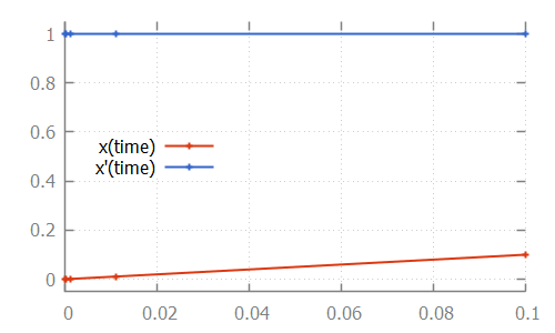
Here, the numerical integrator start with the initial value of continuous
variable x, which is 0.0. For the initial value of variable time,
which is also 0.0, it computes x', which is 1.0. It then slightly
increases the value of variable time to say 1e-6. Assuming a linear
continuous variable x, the value of variable x at that time is 1e-6
as well.
The numerical integrator tries to predict the values of the derivative as time
progresses. It gradually increases the value of variable time, predicting
the value of the derivative at the next time point. If the next prediction
closely matches the actual calculated value, the integrator moves on to the
next time point. If the next prediction is not close enough to the actual
calculated value of the derivative for that time point, more intermediate
values are calculated. That is, the integrator tries to approximate the
derivative as time progresses, while increasing the time between two
consecutive time points. As long as the predictions match the actual
calculated value of the derivative at the next time point, it keeps increasing
the step size even further. If the predictions are not good enough (the
difference with the actual calculated value is above a certain tolerance), more
intermediate time points are investigated. The values calculated for those
time points can then be used to come up with a better approximation, that
better predicts the value of the derivative at future time points.
For the linear ODE given above, the trajectory data calculated by the integrator is:
# time x x'
0.0 0.0 1.0
9.999999999999999e-5 1.0000000000000003e-4 1.0
0.0011 0.0011000000000000005 1.0
0.0111 0.011100000000000006 1.0
0.1 0.10000000000000006 1.0Note that the time points for which the values were calculated, are indicated
in the figure above by small plus signs (+).
The approximations of the integrator don’t need to be linear. Some integrators for instance support nonlinear differential equations. Consider the following CIF specification, with such a nonlinear ODE:
The solution calculated by the numerical integrator is:
cont x = 0.0;
equation x' = (x * x) - x - 2;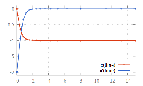
Here, we see how the step size is increased initially, as the linear approximation is good enough. As soon as we get to the bend, the step size is reduced to better approximate the actual values. After the bend, the step size is slowly increased again. The integrator internally uses a polynomial of a higher degree to approximate this differential equation.
If the derivative has a discontinuity, such as in the following CIF specification:
cont x = 1.0;
equation x' = if x < 2: 1.0
else 3.0
end;The integrator will try to figure out the time point at which the discontinuity occurs, by decreasing the step size as it nears the discontinuity. After the discontinuity, the step size is gradually increased, as integration continues:

The basics of numeric root finding
During time transitions, the values of the continuous variables and their derivatives change. If continuous variables or their derivatives are (directly or indirectly) used in guards of edges, changes in their values may result in the guard becoming enabled, as time progresses. To detect such changes during integration, a root finding algorithm can be used.
Consider the following CIF specification:
automaton p:
cont x = 0.0;
equation x' = 0.5;
location:
initial;
edge when x >= 1.5 do x := 0.0;
endHere, the value of continuous variable x increases with 0.5 every time
unit. Once the value of 1.5 is reached, the variable is reset to 0.0.
This process is repeated:

If we look at the data calculated by the numerical integrator, to solve the ODE problem:

we see that values are calculated for time points 1.1111 and 5.0. If we
then also look at the value of the guard, where we use value -1 for
false and +1 for true:
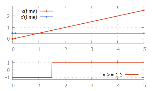
we see that at time 1.1111, the value of the guard is -1 (false).
At time 5.0 it is +1 (true). That is, the guard changed value
between two time points calculated by the integrator. If this is the case, the
ODE solver tries to calculate the exact time point at which the guard changes
its value. That is, it calculates the exact time point at which the guard
function crosses the time axis, and thus has a
root.
One of the simplest root finding algorithms, is the bisection method. This algorithm starts with the two time points where the guard has opposite signs. This is the interval where the guard sign change occurs (it contains the root). The bisection method tries to reduce the size of the interval, by calculating the value of the guard in the middle of the interval. Depending on the sign of the value of the guard at this middle point, this middle point replaces either the lower bound or the upper bound of the interval. This is done in such a way that the values of the guard at the lower and upper bound of the interval have opposite signs, and the interval thus brackets the root.
For the example above, the root is calculated as follows:

We start with the interval [1.1111 .. 5.0]. The middle point is 3.0555 at which
the guard holds, just like the upper bound (at 5.0). Thus 5.0 is replaced by
3.0555. The middle point of 1.1111 and 3.0555 is 1.5972. Since the guard holds
for time 1.5972, upper bound 3.0555 is replaced by 1.5972. The middle point
of 1.1111 and 1.5972 is 1.3542. The guard does not hold at time 1.3542, so the
lower bound of 1.1111 (at which the guard does not hold) is replaced by 1.3542.
This process continues until the interval is smaller than a certain tolerance
value. Once we have that interval, we can choose a value from the interval as
the computed root.
While the bisection method is relatively simple, the root finding algorithms used by the CIF simulator work using the same principles. However, they converge much faster. That is, they requires much less iterations of updating the bounds, to get to a satisfactory answer.
Problems with root finding
With numeric root finding, there is the risk of missing guard changes, which means there is the risk of missing event transitions.
To illustrate the problem, consider the following CIF specification:
automaton p:
cont x = 0.0;
equation x' = 1.0;
location:
initial;
edge when x >= 2.33 and x <= 2.34 do x := 0.0;
endThis specification, when simulated using the CIF simulator, using default settings, results in:
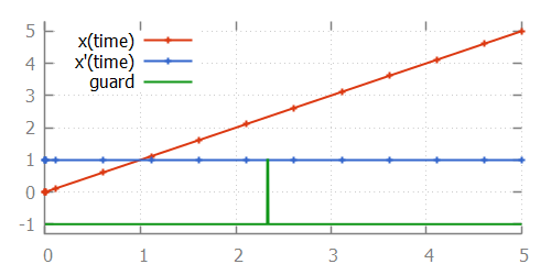
From the image, where the values calculated by the integrator are indicated
using small plus signs (+), we can see that for times 2.1111 and
2.6111, the integrator calculated points. Since the function is linear
between those two time points, no additional intermediate time points were
investigated. Since the guard becomes true after time point 2.1111 (at
time point 2.33) and also becomes false again before time point
2.61111 (at time point 2.34), the integrator misses the guard change.
That is, for every time point that the guard is evaluated, it is false, and
the change in guard value is thus not detected. We miss the guard, and thus
the event that resets variable x to 0.0.
The first solution is to use the
ODE solver root finder maximum check interval
option (ODE solver: ODE root finder
category). This
option can be used to set the maximum time interval between two consecutive
checks of the sign of the guard. By default, this is 0.5 time units. If we
set this value to 0.001, then we ensure that at least once every 0.001
time units, the guard sign is checked. This means that between time points
2.1111 and 2.61111, the guard will be checked approximately 500 times.
This also means that between time points 2.33 and 2.34, the guard will
be checked approximately 10 times. Therefore, this ensures that we check a time
point just before time 2.33, and one just after it, which means we can’t
miss the guard change.
In the above example, x' is 1.0. If however x' would be 2.0,
then the time interval where the guard is enabled reduces from 0.01 time
units to 0.005 time units. Using a maximum check interval of 0.001
would then still suffice, as the guard would be checked approximately 5 times
in that time interval. If however x' is 100, then the time interval
would become 0.0001, which is smaller than the maximum check interval of
0.001. That is, the derivatives of the values occurring in guards influence
the value that should be chosen for the maximum delay interval.
In general, to choose an appropriate value for the maximum check interval, not only the the ranges of values of the variables where the guard is enabled should be taken into account, but the steepness of their derivatives as well. That is, the value of the maximum check interval should be based on the time interval where the guard is enabled. Choosing half the duration of the smallest of such time intervals, for all guards, is generally a good choice.
Note that choosing a smaller interval results in more guard change checks, and thus negatively impacts the performance of the simulation. Therefore, choosing a maximum check interval that is unnecessarily small also unnecessarily reduces performance of the simulation.
We can reformulate the original CIF specification, by splitting the guard:
automaton p:
cont x = 0.0;
equation x' = 1.0;
location:
initial;
edge when x >= 2.33, x <= 2.34 do x := 0.0;
endThis specification, when simulated using the CIF simulator, using default settings, results in:

The difference with the original specification is the guard of the edge. In the
original specification, the and binary operator is used, making it a single
guard. In the new specification, a comma (,) is used, which constructs two
separate guards. Both guards can be individually checked by the root finding
algorithm. As shown in the image, each of the guards changes value only once.
The comma between guards means that both guards have to hold, in order for the
edge to be enabled. This is similar, but not identical, to the and binary
operator. For the and binary operator, the left hand side must be evaluated
before the right hand side, and the right hand side may only be evaluated if
the left hand side evaluates to true. This is called
short-circuit evaluation.
For guards separated by commas, no such relation may be assumed. That is, even if
the first guard evaluates to false, can the second guard still be evaluated by
the root finding algorithm, for guard changes. It can even be the case that the
second guard is evaluated before the first guard. These differences not only
influence root finding, but are also of particular interest when the right hand
side can result in a runtime evaluation failure. For instance, the following
specification:
automaton p:
cont x der 1.0;
location:
initial;
edge when x > 0, 1 / x < 0.5 do x := 0.0;
endresults in a runtime error. The second guard (1 / x < 0.5) is evaluated
even if the first guard (x > 0) does not hold. Initially, the first guard
does not hold, and the second guard results in division by zero. Changing the
comma between the guards to an and operator, makes it possible to simulate
this specification.
Debug information about what the ODE solver calculates, and for what time points, can be enabled using the Debug output option. This may be useful in figuring out why the guard was missed, and what settings need to be changed. See the Debug console output page for more information.
Fixed output step size
The integrator determines the time points for which values are calculated. By default, those points are included in the trajectories. This means that they are also the output of the trajectory data output component. The integrator determines the time points for which to calculate values, based on the complexity of the ODEs. The integrator can be influenced using the integrator options.
Sometimes however, it may be more convenient to have the integration output at more regular intervals. Using the ODE solver fixed output step size option (ODE solver category), a fixed output step size can be configured. This value must be an integer or real number larger than zero.
This option does not influence the actual time points for which the integrator calculates the values. Instead, it influences how these results are put in the trajectories, that are subsequently used by the simulator.
Setting a fixed output step size, ensures that the trajectories contain output for all multiples of the given step size. They will however also contain output for the start and end of each time transition, which may not be at multiples of the step size, due to guards becoming enabled or disabled at other times.
If real-time simulation is enabled, the default is changed to automatically use the model time delta that is used for real-time simulation, as the fixed output step size. This way, the trajectories contain the time points for which intermediate frames are generated. If real-time simulation is enabled, setting a custom fixed output step size is not supported.
Simulation end time and maximum delay
The maximum length of a time transition is determined by several factors:
-
The current simulation time.
-
The simulation end time.
-
The maximum allowed delay amount.
The current simulation time is the value of variable time. Each time
transition starts at the current time.
Using the
Simulation end time
option (Simulator
category), the end time of the
simulation can be configured. By setting a simulation end time, you ensure that
when the value of variable time reaches that value, the simulation
terminates. Settings a simulation end time
also limits the maximum length of a time transition, since from the current
time, a limited amount of time can pass before the end time is reached. By
default the simulation end time is set to 'infinite', which means that
simulation termination, and the maximum length of a time transition, are not
limited by a simulation end time.
Using the
Maximum delay
option (Simulator
category),
the maximum delay amount for a single time transition can be set. If set, no
time transitions longer than the specified value may be calculated. This limits
the maximum length of time transitions to that value. Essentially, this cuts
time transitions into parts with a maximum length specified by this option. By
default, the maximum delay is set to 'infinite', which means that the maximum
length of a time transition is not limited by this option. Restricting the
maximum delay amount for a time transition should generally be avoided.
For debugging purposes however, it may be useful to disable passage of time
altogether. This can be achieved by using a maximum delay of 0.
If both a simulation end time and a maximum allowed delay amount are specified,
the most restrictive of them determines the maximum length of the time
transition. If neither is specified, the simulator will attempt to calculate a
time transition of length 100.0.
ODE solver integrator options
The integrator used by the ODE solver of the CIF simulator, can be configured using several options.
The ODE solver integrator algorithm option (ODE solver: ODE integrator category) can be used to configure the integrator algorithm to use. The following algorithms are available:
-
Higham and Hall 5(4)
-
Dormand-Prince 8(5,3) (default)
-
Adams-Bashforth (experimental)
-
Adams-Moulton (experimental)
The algorithms differ in the complexity of the systems of ODEs that they can handle, their performance, the precision of their results, etc. All these algorithms use an adaptive step size.
The ODE solver integrator absolute tolerance option (ODE solver: ODE integrator category) and the ODE solver integrator relative tolerance option (ODE solver: ODE integrator category), can be used to configure how precise the results of the integrator should be. The lower the tolerance (or error), the higher the precision of the results, but also the more computing time it costs to get to that precision. The absolute precision is the difference between the prediction and the actual value, while the relative precision is that same difference, as a fraction of the actual value. In the latter case, precision reduces with increasing values.
The interval between two consecutive time points calculated by the integrator can be configured using the ODE solver integrator minimum step size option (ODE solver: ODE integrator category) and the ODE solver integrator maximum step size option (ODE solver: ODE integrator category).
The default minimum step size is 1e-15 and the default maximum step size is
0.5. Note however that the last step can be smaller than the value
specified for the minimum step size option.
Increasing the maximum default step size may lead to better performance, but can also lead to less precision, and root finding problems.
The ODE solver integrator number of steps option (ODE solver: ODE integrator category) can be used to configure the number of steps to use for the experimental Adams-Bashforth and Adams-Moulton integrators. The number of steps must be greater or equal to two.
ODE solver root finder options
The root finder used by the ODE solver of the CIF simulator, can be configured using several options.
The ODE solver root finder maximum check interval option (ODE solver: ODE root finder category) is explained on a separate page. See Problems with root finding.
The ODE solver root finding algorithm option (ODE solver: ODE root finder category) can be used to configure the root finding algorithm to use. The following algorithms are available:
-
Regula Falsi (False position) method
-
Illinois method
-
Pegasus method (default)
The Illinois and Pegasus methods are modified Regula Falsi methods. The algorithms differ only in how they choose the middle point of the interval. This influences their convergence speed. The Regula Falsi method in particular should be avoided in practice.
The ODE solver root finder absolute tolerance option (ODE solver: ODE root finder category) and the ODE solver root finder relative tolerance option (ODE solver: ODE root finder category), can be used to configure how precise the results of the root finder should be. The lower the tolerance (or error), the higher the precision of the results, but also the more computing time it costs to get to that precision. The absolute precision is the difference between the prediction and the actual value, while the relative precision is that same difference, as a fraction of the actual value. In the latter case, precision reduces with increasing values.
The ODE solver root finder maximum iterations option (ODE solver: ODE root finder category) can be used to set the maximum number of iterations to use for root finding. This value must be at least one. If the root interval is larger than the tolerances allow, after the maximum number of iterations, root finding fails.
If it fails for your CIF specification, increase the value of this option. If that does not help, your specification is most likely too complex (by nature), or has a modeling error that causes the specification to become too complex for the root finding algorithm to handle. The problem however, may also be in one of the other root finder options, or in one of the integrator options.
Java compiler
The simulator internally generates Java code from the CIF model. This code is compiled using a Java compiler and executed. Code generation and compilation result in faster simulation. However, compilation itself also takes time. The time it takes to compile is different for different Java compilers.
Using the Java Compiler option (Compiler category), the Java compiler implementation to use, can be configured. We currently provide two different Java compilers:
-
Java compiler from the Java Development Kit (
jdk)The Java Development Kit (JDK) that is required to use our tooling includes a Java compiler. This compiler has the advantage that is has a bit less overhead of accessing the file system, while it has as disadvantage that it is a slower in actually compiling the Java code.
-
Eclipse Compiler for Java (
eclipse)The Eclipse Compiler for Java (ecj) is part of the Eclipse Java Development Tools (JDT), and is provided with our tooling. This compiler has the advantage that is is a faster in actually compiling the Java code, while it has as disadvantage that it has a bit more overhead of accessing the file system.
The names given above, in parentheses, indicate the command line option values to use for selecting the different compilers.
In general, the JDK compiler is faster for small CIF models, while the Eclipse compiler is faster for larger CIF models. By default, the JDK compiler is used.
The Java Compiler option has no effect when simulating using a
compiled code file (e.g. a
.cifcode file) for repeated simulations, or when
debugging generated code by enabling
the Load debug code option (Simulator category).
Simulation miscellaneous topics
Complete mode
The CIF simulator calculates for each state the set of transitions that are possible from that state. It is up to the input component to choose one of those transitions, as the transition to take. Using the automatic input mode, it is possible to always choose the first transition that is possible.
In that situation, it is then a waste of resources to calculate the other possible transitions. Using the Complete mode option (Simulator) category), it is possible to enable complete mode. If complete mode is enabled, the calculation of the possible transitions stops as soon as one possible transition is found.
The following values are available for the complete mode option:
-
Auto: disable if possible, enable otherwise
Automatically chooses whether to enable or disable complete mode. If it is allowed to disable complete mode, it will be disabled. Otherwise, complete mode will be enabled.
-
On: forced enabled
Enables complete mode. All possible transitions will be calculated.
-
Off: forced disabled
Disables complete mode. Only the first possible transitions will be calculated.
Currently, it is only allowed to disable complete mode, if the automatic input mode or SVG input mode is used, together with always choosing the first possible transition.
External user-defined functions
The CIF simulator supports external user-defined functions. Currently, the following external languages are supported:
Asynchronous execution
By default, external user-defined functions are executed asynchronously. This ensures that the simulation can be terminated during the execution of such a function. This is useful if such functions take a long time to execute. It is also particularly useful for external functions that never terminate, for instance because they get stuck in a loop, often due to a bug.
This asynchronous execution however, does lead to a performance penalty. To get rid of this performance penalty, disable asynchronous execution, leading to synchronous execution. Asynchronous execution can be disabled using the External functions asynchronous execution option (Simulator category).
By disabling the asynchronous execution, the simulator can no longer be terminated if it gets stuck executing an external user-defined function. If the functions runs for a long time, the termination is postponed until the external function finishes its execution.
Side effects
All user-defined functions in CIF are pure mathematical functions. They must therefore be deterministic, and may not have side effects. For internal user-defined functions, this is enforced. For external user-defined functions, it is mostly impossible to check this constraint in an implementation, and the responsibility for checking this is therefore delegated to the end user. Practically, this means that for instance logging statements in functions, while essentially side effects, may be permitted, as long as the function returns the same value, if given the same arguments. This is essential for correct simulation results, as the results of function calls may for instance be cached by the simulator.
Value semantics
The CIF simulator uses value semantics for the parameters and return values of functions. That is, changes to the parameters of functions in external user-defined functions are not reflected back to the CIF specification. Furthermore, changes to the return values in the CIF simulator have no effect on subsequent calls to external user-defined functions.
External user-defined Java functions
External user-defined Java functions allow the use of static Java methods from CIF specifications. This page explains how to use such Java methods, how the simulator loads and invokes them, what is allowed, etc. It explicitly does not explain how to write or compile Java code.
External implementation reference
Consider the following examples of external user-defined Java function:
func real f1(real x): "java:java.lang.Math.expm1";
func int f2(bool x): "java:pkg.Cls.method|../some.jar;bin";Two external user-defined functions are given as examples. Both have a string
literal as external implementation reference. For Java functions, the string
literal must start with java:. Then the absolute name of the Java method
that is to be invoked is given. That is, the package name, class name, and
method name are given, separated by dots (.).
Optionally, a Java class path may be given at the end, preceded by a bar
(|) character. The class path entries must be separated by semicolons
(;) regardless of the operating system. The class path entries are absolute
or relative local file system paths to Jar files or directories with Java class
files. Relative paths are resolved against the directory that contains the
CIF specification in which the external user-defined function is declared. Both
Linux/Mac path separators (/) and Windows path separators (\) may be
used in class path entries. However, \ must be escaped as \\ in CIF
string literals, and thus it is recommended to always use / as path
separator. A discussion of the Java class path concept is beyond the scope of
this documentation.
Supported types and values
Not all CIF data types are supported for the parameters and return values of external user-defined Java functions. The following table lists the allowed CIF types, and their corresponding Java types.
| CIF type | Java type |
|---|---|
|
|
|
|
|
|
|
|
|
|
|
|
|
|
|
|
|
|
Unless otherwise specified, the primitive Java types (boolean, int,
and double) can be used interchangeably with their class variants
(java.lang.Boolean, java.lang.Integer, and java.lang.Double).
For lists and sets, the element type recursively affects the type parameters of
the Java types. Similarly, for dictionaries, the key and value types affect
the type parameters of the Java Map type. Since Java doesn’t have tuples,
and there is no way in Java to define a type with a variable number of type
parameters, CIF tuples are passed to Java as a list of objects. It may be
assumed that such lists have the same number of elements as there are fields in
the original tuple, and that the elements have types that correspond to the
types of the field of the tuple. The following table shows a few examples:
| CIF type | Java type |
|---|---|
|
|
|
|
|
|
|
|
For parameters, no null values are ever passed, not even as elements of
lists, etc. Furthermore, for real typed values, NaN, positive infinity,
and negative infinity are never passed along.
For return values, null values, as well as NaN, positive infinity, and
negative infinity are considered runtime errors. Furthermore, integer values
outside their CIF integer type range bounds are considered runtime errors as
well.
Method resolution
The class as specified in the external implementation reference is loaded using a Java class loader. By default, the system class loader is used. If additional class path entries are specified in the external implementation reference, an extended class loader is used that searches in the additional class path entries before deferring to the system class loader. The class is loaded using the binary name of the class.
The method that is resolved must be a static method. The access modifier of the
static method is irrelevant. That is, it doesn’t matter whether the method is
private, protected, public, etc.
The method is resolved in the Java Virtual Machine (JVM) that runs the
simulator. The method is resolved by name, and parameter types. The parameter
types only include the top level type. That is, for CIF type list int, the
Java type java.util.List is used as the type of the parameter. If more than
one method with the same parameter types is declared in the class, and one of
these methods has a return type that is more specific than any of the others,
that method is used. Otherwise one of the methods is chosen arbitrarily.
For parameters that have primitive Java types as their type, the primitive
types are used to resolve the method instead of their classes. In other words,
when resolving the method, or the proper overload of the method, int and
java.lang.Integer are considered incompatible.
The CIF simulator employs lazy loading. That is, if the external Java function is never called, it is also never loaded.
Method invocation
The method is invoked in the Java Virtual Machine (JVM) that runs the simulator, using reflection. By default, it is invoked asynchronously.
Since the parameter types are not checked recursively when the method is resolved, methods may fail to execute properly if the type signatures don’t match exactly. Similarly, for the return type only the top level type is checked. If a return value does not match the CIF type (wrong element type, wrong tuple length, etc), simulation will fail with a runtime error.
Any exceptions that occur during execution of the Java method are caught by the simulator. When the simulator catches such an exception, it will print the Java stack trace of the exception to the console, and simulation will be terminated.
Side effects
As all functions in CIF, external user-defined Java functions should not have any side effects. That is, if called with the same arguments, it should return the same value each time. More concretely, maintaining state information should be avoided, as should file I/O, and reading from stdin.
Writing to stdout and stderr should not affect the result of the method. It should however be avoided as well, as such writes are associated with the streams of the Java Virtual Machine (JVM), and not the simulator. The output will not end up on the Eclipse console of the simulator.
By default, the Java methods are invoked asynchronously, on a freshly created thread. That is, there is no guarantee that an invocation uses the same thread as the previous invocation. If static fields (class variables) are used to maintain state, this may cause problems if thread safety is not ensured by the Java method. If synchronous execution is used, all external function calls are invoked from the simulation thread, and such thread safety issues should not be a problem.
You should assume that each external function is loaded using a different class loader. As such, multiple Java methods from the same class, from the same external library, may be loaded using different class loaders as well. As such, shared static fields (class variables) of those classes can in general not be shared by different external functions.
Profiling
The CIF simulator has a Profiling option (Simulator category). If the option is enabled, information about the number of transitions taken per second, is printed to the console. Enabling profiling disables most other types of console output. By default, profiling is disabled.
The profiling output looks somewhat like this:
750431.42 transitions/second
640589.87 transitions/second
890939.01 transitions/second
887228.57 transitions/second
890143.25 transitions/second
893674.44 transitions/second
891812.69 transitions/secondStochastic distributions and seeds
Stochastics can be used to model randomness in CIF models. The CIF simulator exhibits pseudo-randomness. This page explains how to influence that pseudo-randomness.
The randomness of the stochastic distributions is implemented in the CIF simulator using pseudorandom number generators (PRNGs). The PRNG used is the Mersenne Twister. The sequences of random numbers that are generated by the MT are not truly random. They are pseudorandom, as they start to repeat after some time. The Mersenne Twister however, has a very long period of 219937 - 1 numbers.
Since the sequence of generated random numbers is always the same, the only way to vary it, is to use a different starting place. The starting place is determined by the initial seed, which can be configured through the Initial seed for stochastic distributions option (Simulator category). If specified, it must be a value in the range [1 .. 230]. If it is not specified, a random initial seed in that range is chosen by the simulator. If a random initial seed is chosen, and it is used, it is printed to the console.
The initial seed as provided by the option, is used for the first stochastic distribution that is created. Each subsequent distribution uses the next available seed. That is, if you specify an initial seed of 5, then the first distribution is created with an initial seed of 5, the next one uses 6, the third one uses 7, etc. The initial seeds are kept in the range [1 .. 230]. After seed 230, 1 is used as seed, then 2 is used as seed, etc.
Simulating the same specification multiple times, using the same initial seed, results in the same samples. Therefore, using a fixed seed can make your simulation deterministic, even though you use stochastic distributions to introduce randomness into your specification.
Simulation developer topics
Maximum time point tolerance
| This page is primarily intended for the developers of the CIF simulator, and not its end users. |
The CIF simulator internally often queries the trajectories computed by the ODE solver. Due to the limited precision of binary floating point number representations, requests of time points for which no exact match is present in the trajectories, but for which a very close match is present, are allowed. The simulator compensates for these small deviations, to avoid accumulation of such deviations.
The simulator uses the value of the Maximum time point tolerance option (Simulation category) to determine whether two time points are close enough to each other to constitute a match. The tolerance is given in ulps (units in the last place, or units of least precision). One ulp is the difference between two subsequent floating point numbers, for the limited precision binary floating point number representation used by the simulator. That is, two floating point numbers are one ulp away from each other, if there is no other floating point number between them, that can be represented using the floating point number representation used by the simulator. Since an ulp increases as the floating point numbers increase, the tolerance is thus relative to the values of the time points.
The tolerance values chosen using the option must be in the range [1 .. 230]. The default tolerance is 210 (= 1024) ulps. The default tolerance should suffice, but if it doesn’t, you may be presented with an error like this:
ERROR: Simulation resulted in a runtime error, for state: time=0.0, x=1.0.
CAUSE: Requested time point "1.6000000000000005" is "2.0" ulps (1 ulp = 2.220446049250313e-16) away from the closest time point in the trajectories "1.6", which is farther away than the maximum tolerance of "1" ulps. You can try increasing the value of the maximum time point tolerance option. Please also contact the development team.If you get such an error, you can try to increase the tolerance using the Maximum time point tolerance option, in order to be able to continue your simulation. However, as this shouldn’t actually happen, you should also contact the development team, who will then figure out why the default tolerance doesn’t suffice for your model.
Debugging generated code
| This page is primarily intended for the developers of the CIF simulator, and not its end users. |
The CIF simulator generates highly optimized code for the specification, to speed up the simulation. By enabling the Debug the generated code (by writing it to disk) debugging output, the generated code can be written to disk, for further debugging.
Output directory
If the simulation is performed from within Eclipse, and a project named
org.eclipse.escet.cif.simulator.debug exists, is not closed, and has a src
directory, the generated code will be written to that src directory.
Otherwise, the generated code will be written to the directory containing the
input specification file.
Regardless, the code is also always written to a cifcode
sub-directory. If this sub-directory does not yet exist, it is created. If it
already exists, all existing .java files are removed from the
sub-directory first, before the newly generated code is written.
Written files
The generated code consists of Java files only. This results in several
.java files being written to the cifcode directory.
Additionally, an Eclipse launch configuration file (_cifsim_debug.launch)
is written. This launch configuration can be used to reproduce the simulation
implemented by the generated code. The launch configuration
reproduces the simulation options that were used, and always shows the option
dialog. The working directory for the simulation performed via the generated
launch configuration is the same working directory as the original simulation.
This allows additional files, such as configuration files, to be found.
How to use
To use this feature, follow these steps:
-
Import all CIF related source projects into your Eclipse workspace.
-
Make sure your workspace is automatically rebuilt, by enabling the Build Automatically option in the Project menu.
-
Start a sub-Eclipse application, by right clicking on any plug-in project in the workspace, and choosing or .
-
In the sub-Eclipse that opens, make sure the CIF specification (the
.ciffile) that you like to simulate is available in the workspace. -
In the sub-Eclipse, import the
org.eclipse.escet.cif.simulator.debugsource project. -
Simulate the CIF specification, and make sure you enable the Debug the generated code option.
-
Continue simulation, if desired.
-
Once the simulation has terminated, switch back to the main Eclipse.
-
Refresh the
org.eclipse.escet.cif.simulator.debugproject. -
Set breakpoints in the generated Java code, or in the simulator code, as desired.
-
Right click the launch configuration in the
src/cifcodedirectory, and choose . -
Debug the simulation, with the generated code, as you would any Java program.
Starting the simulator with generated code
The launch configuration that is written to disk with the generated code, uses the Load debug code option (Simulator category). Using this option, the classpath (directory) where the already generated code is located, is specified. By specifying it, the simulator knows from where to load it.
Simulations not started from the generated launch configuration, generally don’t use this option. They load the input specification, validate it, generate fresh code, and compile the code in-memory, or use compiled code files
Simulations using the generated code ignore all options related to repeated simulations. That is, the Load debug code option takes priority over the Compile only option (Compiler category), and simulating with compiled code files.
A warning is printed to the console if the generated code was generated with a different version of the simulator than the one used to simulate it. Ignoring the warning may lead to unexpected simulation results, or even simulator crashes.
Test mode
| This page is primarily intended for the developers of the CIF simulator, and not its end users. |
In order to be able to perform automated testing, the Test mode option (Output category) can be used. This option has the following effect:
-
The visual interfaces for all output components (such as visualizers) are disabled.
-
The user is no longer asked to confirm termination of the simulator, if the the Ask to confirm simulator termination option (Simulator category) is configured to let the simulator decide whether to ask the user for confirmation or terminate automatically. By not asking for user input at the console, the automated test set can be fully automatically executed.
-
It is allowed to perform real-time simulation without using any real-time output components, allowing testing of the real-time functionality in the automated test set.
-
All real-time delays are skipped. By not performing unnecessary real-time delays, the automated test set executes as fast as possible.
-
SVG visualization operates in synchronous mode, rather than asynchronous mode. This ensures that debug output becomes synchronous as well, and we thus get consistent output for our test cases. This is not only useful for automated testing, but also for debugging.
Verification tools
CIF to mCRL2 transformer
The CIF to mCRL2 transformer is used to convert a CIF specification to a mCRL2 specification. mCRL2 is a tool for verifying properties of the model.
Starting the transformation
The transformation can be started in the following ways:
-
In Eclipse, right click a
.ciffile in the 'Project Explorer' tab or 'Package Explorer' tab and choose . -
In Eclipse, right click an open text editor for a
.ciffile and choose . -
Use the
cif2mcrl2tool in a ToolDef script. See the scripting documentation and tools overview page for details. -
Use the
cif2mcrl2command line tool.
Options
Besides the general application options, this application has the following options:
-
Input file path: The absolute or relative file system path to the input CIF specification.
-
Instance tree definition: mCRL2 uses a tree of processes which you can specify manually here. If not specified, it takes the default solution, which first merges all CIF automata (one at a time), and on top of that, the variable processes of the shared variables (also one at a time). How to define your own tree is explained in the instantiation tree syntax Section.
-
Enable debug output: The transformer derives information about used and available variables in the instantiation tree, and uses that information to generate the mCRL2 action operations at every level. By enabling this option, this information is also written to an output file for further external analysis. By default, the information is written in a file with the same name as the input file, except first the
.cifextension is removed (if present), and a_dbg.txtextension is appended. The name of the output file can be changed with the Debug output file path option. Setting the latter option enables this option. -
Debug output file path: The absolute or relative file system path to use for writing derived information about used and available variables at every level in the instantiation tree. Setting this option changes the debug output file path to the given path. It also enables the Enable debug output option.
-
Output file path: The absolute or relative file system path for writing the generated mCRL2 output file. By default, the output file path is the same as the input file path, but with the
.cifextension removed (if it exists), and the.mcrl2extension added. By setting this option, the default is overridden by the given value. -
Generate 'value' actions: To query the value of variable
x, avalue_xaction can be used. By default, such actions are generated for every variable in the system. Using this option, you can define precisely which variables should have such an action. See the Generation of 'value' actions Section for more details.
Supported specifications
The CIF to mCRL2 transformer supports a subset of CIF specifications. The following restrictions apply:
-
The transformer ignores the supervisory kind of the automata.
-
Algebraic variables are not supported.
-
Continuous variables are not supported.
-
Equations are not supported.
-
Initialization predicates are not supported, except for initialization predicates in a location.
-
Invariants are not supported.
-
Marker predicates are ignored.
-
Discrete variables must have type
boolorint. The latter may have a range. -
Multiple potential initial values are not supported.
-
Initial value must be a constant.
-
There must be at least one automaton.
-
The transformation translates the range of integer variables if used, but it does not enforce the maximum and minimum integer value of CIF.
In automata, there are a number of extra conditions:
-
The
initialexpression in locations must be constant. -
There must be a single initial location in each automaton.
-
Conditional updates are not supported, only assignment updates are allowed.
-
Multi-assignments are not supported.
-
Channels are not supported.
-
The
tauevent is not supported. -
Urgency of locations and edges is ignored.
-
Location references are not supported.
-
All expressions and sub-expressions must be of type
boolorint. The latter may have a range. -
Boolean constants, discrete variables, and operators
and,or,==,>=,>,<=,<,!=, andnotare allowed. -
Integer constants, discrete variables, binary operators
+,*,-, and unary operators-and+are allowed.
However, some of these limitations are resolved by preprocessing of the specification, as explained in the next section.
Preprocessing
The following CIF to CIF transformations are applied as preprocessing (in the given order), to increase the subset of CIF specifications that can be transformed:
Generation of 'value' actions
The CIF to mCRL2 transformer generates a value action for each variable by
default. In some cases, this may not be wanted. Variables that never have to
be queried for their value do not need such an action. Having such an action
available anyway increases the amount of work that has to be done by the mCRL2
tool. To eliminate these unneeded value actions, the CIF to mCRL2
transformer has the Generate 'value' actions option.
The option takes a comma separated list of variable patterns. Each pattern
can add or remove variables. If the pattern starts with a + character,
variables are added. If the pattern starts with a - character, variables
are removed. If the pattern start neither with a + nor with a -
character, variables are added. The main part of each pattern is the name of
the variable to add or remove. In addition, you can use the * character
as a shorthand for 'zero or more arbitrary characters', allowing you to write
abbreviations, and match several variables at the same time.
For example, assume existence of the following variables in a CIF model:
A.p12 A.q2 A.z B.x B.y1 B.y2 B.z C.qBelow a number of example option values, and what variables they select from the above list.
-
The option value
B.x,+A.zselects variablesB.xandA.z. -
The option value
+*1matches all variables that end with a1, which is variableB.y1only (VariableA.p12does have a1in it, but not at the end.) -
The option value
+*1*matches all variables with a1at any position. This matches bothA.p12andB.y1. -
The option value
+*,-B.*selects all variables, except those in automatonB. (*adds all variables, then-B.*removes all variables that start withB., that is all variables in automatonB.) -
The option value
-*removes allvalueactions, since the pattern removes all variables.
Syntax of the instance tree
In mCRL2, a behavior process is required for every automaton in the input, and a variable process is needed for every variable used (read or written) by two or more automata. In addition, it is allowed to have a variable process for variables that are used in one automaton only (that is, a local variable of the automaton).
All these processes must be instantiated using the parallel composition operator. For larger specifications, the naive solution of instantiating all processes together in one level fails due to having too many allowed combinations of actions for the mCRL2 tool to handle.
A different solution is to instantiate smaller groups of processes at a time, and then use these groups again in other instantiations. Instantiation happens in multiple levels in this case, leading to a tree of process instantiations. At each level, the set of allowed actions is restricted by adding action operators. This results in a large reduction of the number of possible combinations of actions that need to be explored by the mCRL2 tool. Fewer combinations of actions in turn leads to enabling larger specifications to be verified.
Which processes and groups are taken together at each level in the tree has a large impact on feasibility. The CIF to mCRL2 transformer has a default scheme, where pairs of one group and one behavior process are taken together at each level (except at the bottom, where two behavior processes are merged instead). On top of that tree, pairs of a group and a variable process are taken together.
The CIF to mCRL2 transformer does not perform analysis to decide how processes and variables should combined. In many cases this provides a working solution. For some specifications however, you may want to have more influence in the order of grouping. For this reason, the Instance tree definition option exists. It allows you to define which processes should be taken together at each level in the instantiation tree.
The current implementation has limits with respect to ordering. Automata processes must be merged first (but the number of levels and the order of combining is free), and then variables must be added one at a time (but which variable to use at each level is free).
The option expects absolute names of all automata in the specification and absolute names of all discrete variables used in two more automata, separated by white space or commas. In addition you may add the absolute names of variables used in only one automaton. For each element mentioned, a process is created in mCRL2. Variables used in one automaton that are not mentioned, become local variables of the behavior process of the automaton that uses the variable.
Processes for the mentioned CIF elements are instantiated. Sub-groups of processes are written by surrounding them with parentheses. For example:
( ( A B C ) A.x ) B.ytakes automata A, B, C together. One level higher, variable
A.x is added, and finally variable B.y is added at the highest level.
Another order is:
( ( ( A B ) C ) B.y ) A.xFirst processes A and B are combined, then process C is added, and
finally variables B.y and A.x at the top-most two levels.
Debug output
The transformer analyzes use of the variables by each automaton, and computes variable usage and availability of the variables at each level in the instantiation tree. This information is written to a file with debug output by enabling the Enable debug output option. As an example, consider the following artificial CIF specification:
event a, b, c;
automaton P:
disc int[0..10] x = 0;
disc int[-5..5] zero = 0;
location p1:
initial;
edge a do x := x + 1 goto p2;
location p2:
edge c when Q.y != 0 goto p1;
edge a do x := 1 goto p1;
end
automaton Q:
disc int[0..1] y = 1;
location q1:
initial;
edge a when y = 1 goto q2;
location q2:
edge b when y = 1 and P.x < 8 and P.zero = 0 goto q1;
endThis specification has two automata P and Q, and two shared variables
P.x and Q.y. The ranges of the variables are important, mCRL2
considers the integer type unbounded, depending on your CIF file, without
giving upper and lower bounds for the variables, you may end up in the
situation that mCRL2 tries every single value of its infinite integer type,
which takes a very long time!
Variable zero is not shared, only automaton Q uses it. The transformer
moves it to the Q process. Normally however, you would use a constant
instead of a variable.
The instance tree used in the transformation is ( ( P Q ) P.x ) Q.y. The
debug output for P is:
===============================================================
Node 1.1.1.1
Variable use by behavior processes ordered by event:
a:
P.x read:SOMETIMES write:ALWAYS
c:
Q.y read:ALWAYS write:NEVERAutomaton P has one c edge, which checks the value of Q.y but it
does not change its value. It has two a edges, only the a edge in
location p1 reads P.x (to compute x + 1). Both edges assign a new
value to P.x.
In a similar way, the node information for automaton Q is computed. The
result is:
===============================================================
Node 1.1.1.2
Variable use by behavior processes ordered by event:
a:
Q.y read:ALWAYS write:NEVER
b:
Q.y read:ALWAYS write:NEVER
P.x read:ALWAYS write:NEVERThe automaton only checks values rather than writing them. As you can see,
variable P.x is not mentioned with event a, since there is no edge in
the automaton with event a that accesses variable P.x.
The node that merges both automata, i.e. ( P Q ), has the following
formation:
===============================================================
Node 1.1.1
Variable use by behavior processes ordered by event:
a:
P.x read:SOMETIMES write:ALWAYS
Q.y read:ALWAYS write:NEVER
c:
Q.y read:ALWAYS write:NEVER
b:
Q.y read:ALWAYS write:NEVER
P.x read:ALWAYS write:NEVER
Children:
node 1.1.1.1
node 1.1.1.2Variable use by each event is simply merged. In this example there is no
overlap, but that works as you would expect, SOMETIMES overrides
NEVER, and ALWAYS overrides SOMETIMES.
The node for variable process for P.x only provides a variable:
===============================================================
Node 1.1.2
Available variable processes:
P.xThe output states that variable P.x is available here.
At ( P Q ) P.x node, the merge of the variable P.x with the two
automata, this results in:
===============================================================
Node 1.1
Available variable processes:
P.x
Variable use by behavior processes ordered by event:
a:
P.x read:SOMETIMES write:ALWAYS
Q.y read:ALWAYS write:NEVER
c:
Q.y read:ALWAYS write:NEVER
P.x read:NEVER write:NEVER
b:
Q.y read:ALWAYS write:NEVER
P.x read:ALWAYS write:NEVER
Children:
node 1.1.1
node 1.1.2In this node, variable P.x is also available. The variable process does
not perform events, so the event variable table of node 1.1.1 is copied.
The only exception is the additional line P.x for event c. The reason
for this line is that while ( P Q ) may not use P.x in combination
with event c, other automata higher up in the tree may still need that
variable. (In a future version of the transformer tool, it may be detected
that such use never happens, and there is no need to add the line here.)
Node 1.2 is the variable process of Q.y. It looks the same as node
1.1.2, except for the name of the variable.
Finally the top-node that merges ( P Q ) P.x with Q.y, bringing
everything together, looks like:
===============================================================
Node 1
Available variable processes:
P.x
Q.y
Variable use by behavior processes ordered by event:
a:
P.x read:SOMETIMES write:ALWAYS
Q.y read:ALWAYS write:NEVER
c:
Q.y read:ALWAYS write:NEVER
P.x read:NEVER write:NEVER
b:
Q.y read:ALWAYS write:NEVER
P.x read:ALWAYS write:NEVER
Children:
node 1.1
node 1.2The Q.y variable is now also available. The event variable table is again
copied. Since all events already used variable Q.y no additional lines
were added.
Output of the transformation
A variable process in mCRL2 handles shared access to a variable. For variable
P.x in the above example it looks like:
act value_x, vread_x, vwrite_x, sync_x, aread_x, awrite_x : Int;
proc VarProc_x(v:Int) =
value_x(v) . VarProc_x(v) +
vread_x(v) . VarProc_x(v) +
sum m:Int . ((m >= 0) && (m <= 10)) -> vwrite_x(m) . VarProc_x(m) +
sum m:Int . ((m >= 0) && (m <= 10)) -> vread_x(v) | vwrite_x(m) . VarProc_x(m);The name of the actions all end with the name of the variable. If the CIF specification has two or more variables with the same name, a number gets appended to make each variable unique in mCRL2.
A behavior process is generated for each automaton instance. Like the variables, the name of the automaton is used in the output. If there are name conflicts, a number is appended to make it unique. The process is the same list of edges of the original CIF automaton, with added read and write actions for synchronizing with the variable processes:
sort LocSort_P = struct loc_P_p1 | loc_P_p2;
proc BehProc_P(Locvar_P : LocSort_P) =
sum x : Int . ((x >= 0) && (x <= 10) && (Locvar_P == loc_P_p1)) -> a | aread_x(x) | awrite_x((x + 1)) . BehProc_P(loc_P_p2) +
sum y : Int . ((y >= 0) && (y <= 1) && (Locvar_P == loc_P_p2) && (y != 0)) -> c | aread_y(y) . BehProc_P(loc_P_p1) +
(Locvar_P == loc_P_p2) -> a | awrite_x(1) . BehProc_P(loc_P_p1);Locations are encoded in a struct and variable read and write actions are
added as needed.
The instantiation tree is dominated by the action operators needed for
synchronizing and restricting actions. The value_... actions are allowed
up the to top level node, to give access to variable values in the
verification. This leads to:
act a, renamed_a, c, renamed_c, b, renamed_b;
init block({aread_y, awrite_y, vread_y, vwrite_y},
hide({sync_y},
comm({aread_y | vread_y -> sync_y,
awrite_y | vwrite_y -> sync_y},
(
block({aread_x, awrite_x, vread_x, vwrite_x},
hide({sync_x},
comm({aread_x | vread_x -> sync_x,
awrite_x | vwrite_x -> sync_x},
(
allow({value_zero,
a | awrite_x | aread_y,
a | awrite_x | aread_x | aread_y,
c | aread_y,
b | aread_y | aread_x},
rename({renamed_a -> a},
block({a},
comm({a | a -> renamed_a},
(
BehProc_P(loc_P_p1)
||
BehProc_Q(loc_Q_q1, 0)
)))))
||
VarProc_x(0)
))))
||
VarProc_y(1)
))));CIF to UPPAAL transformer
The CIF to UPPAAL transformer can be used to transform CIF specifications
to UPPAAL systems (*.xml files).
UPPAAL
is a tool modeling, validation, and verification of networks of timed automata with
variables. The transformer only transforms untimed CIF specifications.
Starting the transformation
The transformation can be started in the following ways:
-
In Eclipse, right click a
.ciffile in the 'Project Explorer' tab or 'Package Explorer' tab and choose . -
In Eclipse, right click an open text editor for a
.ciffile and choose . -
Use the
cif2uppaaltool in a ToolDef script. See the scripting documentation and tools overview page for details. -
Use the
cif2uppaalcommand line tool.
Options
Besides the general application options, this application has the following options:
-
Input file path: The absolute or relative local file system path to the input CIF specification.
-
Output file path: The absolute or relative local file system path to the output UPPAAL file. If not specified, defaults to the input file path, where the
.ciffile extension is removed (if present), and a.xmlfile extension is added.
Supported specifications
The CIF to UPPAAL transformer supports a subset of CIF specifications. The following restrictions apply:
-
Specifications without automata are not supported.
-
Channels (events with data types) are not supported.
-
Initialization predicates in components are not supported.
-
Automata that do not have exactly one initial location are not supported.
-
Locations with initialization predicates that are too complex to evaluate statically, are not supported. That is, those predicates must essentially be be constant. For instance,
trueandtrue or falseare supported, as iscifcis a constant. However,v => cwithva discrete variable that can initially have several different values, is not supported. -
Discrete variables with multiple potential initial values are not supported.
-
Discrete variables with initial values that are too complex to evaluate statically, are not supported. That is, their initial values must essentially be constant. For instance,
1 + 1and2 * 5are supported, as isc + 1ifcis a constant. However,v * 2withva discrete variable that can initially have several different values, is not supported. -
Enumerations are not supported.
-
Continuous variables are not supported.
-
Algebraic variables are not supported.
-
Input variables are not supported.
-
User-defined functions are not supported.
-
Urgent edges are not supported.
-
Multi-assignments on edges (such as
do (x, y) := (1, 2)) are not supported. However, it is allowed to use multiple assignments on an edge (such asdo x := 1, y := 2). -
Partial variable assignments (such as
do x[0] := 5) are not supported. -
Conditional updates (
ifupdates) on edges (such asdo if b: x := 5 end) are not supported. -
Only the following data types are supported: boolean types and integer (both with a range and without a range).
-
Only the following expressions are supported: boolean literal values (
trueandfalse), integer literal values, binary expressions (partially, see below), unary expressions (partially, see below), casts that don’t change the type,ifexpressions, and references to constants, discrete variables, and locations. -
Only the following binary operators are supported: logical equivalence (
<=>), logical implication (=>), logical conjunction (andon boolean operands), logical disjunction (oron boolean operands), addition (+) on integer operands, subtraction (-) on integer operands, multiplication (*) on integer operands, integer division (div), integer modulus (mod), equality (=) on integer operands, inequality (!=) on integer operands, less than (<) on integer operands, less than or equal to (<=) on integer operands, greater than (>) on integer operands, and greater than or equal to (>=) on integer operands. -
Only the following unary operators are supported: logical inverse (
not), negation (-) on an integer operand, and plus (+) on an integer operand. -
Only state invariants are supported. State/event exclusion invariants are not supported. To allow state/event exclusion invariants to be used in the input, manually eliminate them first using the Eliminate state/event exclusion invariants CIF to CIF transformation.
-
The controllability of events is ignored.
-
The supervisory kinds of automata are ignored.
-
The supervisory kinds of invariants are ignored.
-
Marker predicates are ignored.
Preprocessing
The following CIF to CIF transformations are applied as preprocessing (in the given order), to increase the subset of CIF specifications that can be transformed:
Transformation result
CIF features synchronizing events, while UPPAAL only supports channels. A
SendAut automaton/template is added to the UPPAAL system to ensure proper
event synchronization. The UPPAAL template has a single location, and self
loops for every event in the CIF specification. The guards of the self loops
express the conditions under which the events are globally enabled (guard wise)
in the CIF specification. Every CIF event is a broadcast channel in UPPAAL. If
the self loop is enabled (guard wise), the SendAut template broadcasts over
the channel. All the other templates (for the CIF automata) receive the event.
They can actually receive, as the guard of the self loop ensures that. Together
the SendAut self loops and the receive edges form the synchronization.
As the SendAut template needs to refer to locations of the other templates,
location pointer variables are added for all the other templates. For every
CIF automaton some.aut, a location pointer variable LP_some_aut is
added. The location pointers are integer variables with range [0,n-1], for
an automaton with n locations. Updates are added to the edges to ensure the
location pointer variables have the proper values. The location pointers are
similar to those created by the CIF to CIF transformation that
eliminates the use of locations in expressions.
In CIF, assignments interpret the right hand side of the assignment (the new
value of the variable) in the source state of the transition. In UPPAAL,
assignments have order, and the right hand sides are interpreted over the
current state, after any preceding assignments. Furthermore, the order in which
the assignments of the edges of different participating templates are executed
is not defined. To ensure the proper CIF semantics, 'old' versions of all
variables (including the location pointer variables) are added. For a variable
x, OLD_x is added. The SendAut automaton assigns the current values
of all variables to their 'old' counterparts. The assignments on the edges of
the other automata then use the 'old' variables to compute the new values of
the variables. As the values of the 'old' variables are only used during the
transitions, the 'old' variables are meta variables in the UPPAAL system.
The invariants from CIF components are added to the location of the SendAut
template.
For CIF variables with an int type, the UPPAAL type is
int[-2147483648,2147483647].
The names of templates, variables, etc in UPPAAL are based on the absolute
names of their CIF counterparts. For a variable a.b.c in CIF, the UPPAAL
name is a_b_c. If there are conflicts between the UPPAAL names, or if one
of the UPPAAL names conflicts with a UPPAAL keyword, renaming is performed, and
a warning is printed to the console.
No geometry is generated. When the generated UPPAAL file is opened in UPPAAL, UPPAAL will perform some layouting.
Real-time testing, code generation, and implementation tools
CIF code generator
The CIF code generator can be used to generate implementation code for various languages/platforms. The generated code is complete, and can be used as is, without any CIF related library or runtime.
The remainder of this page explains general information about the tool, that applies to all target languages/platforms. Specific information is available for each of the target languages/platforms, on separate pages:
-
C89 (if there is no
C99compiler) -
Simulink, with an example of controlling a tank
Starting the generator
The generator can be started in the following ways:
-
In Eclipse, right click a
.ciffile in the Project Explorer or Package Explorer and choose . -
In Eclipse, right click an open text editor for a
.ciffile and choose . -
Use the
cifcodegentool in a ToolDef script. See the scripting documentation and tools overview page for details. -
Use the
cifcodegencommand line tool.
Options
Besides the general application options, this application has the following options that apply to all target languages/platforms:
-
Input file: The absolute or relative local file system path to the input CIF specification.
-
Output directory: The absolute or relative local file system path to the output directory. This is the directory to which the generated code files will be written. If the directory does not yet exist, it is automatically created. By default, the current directory is used.
-
Target language: Specifies the target language/platform for which to generate code. By default, C99 code is generated. The following languages/platforms are supported:
Target language/platform Command line value c89c99javasimulinkThe first column indicates the target language/platform, and is linked to a page with more information for that specific language/platform. The second column indicates the command line value to use for the option, to select that target language/platform.
-
Code prefix: The code prefix, used to prefix file names, identifiers in the code, etc. If no prefix is given, the prefix is derived from the input filename, by removing the
.ciffile extension, if present. This is also the default. The prefix must be a valid CIF identifier, i.e. consist of only letters (atoz,AtoZ), numbers (0to9), and underscores (_), and not start with a number.
Supported specifications
The CIF code generator supports a subset of CIF specifications. The following restrictions apply:
-
Specifications without automata are not supported.
-
Initialization predicates in components are not supported, except if it can be determined statically that they are trivially
true. -
State invariants in components are not supported, except if it can be determined statically that they are trivially
true. -
State/event exclusion invariants (in components as well as locations) are not supported. To allow state/event exclusion invariants to be used in the input, manually eliminate them first using the CIF to CIF transformation.
-
Discrete variables with multiple initial values (including
any) are not supported. -
External user-defined functions are not supported.
-
Urgent locations are not supported.
-
Initialization predicates in locations that can not be statically evaluated are not supported.
-
State invariants in locations are not supported, except if it can be determined statically that they are trivially
true. -
Automata that do not have exactly one initial location are not supported.
-
Urgent edges are not supported.
-
Data types other than
bool,int(with or without range),real,string, enumerations, tuples, and arrays, are not supported. This applies to the data types of variables, parameters of functions, return types of functions, etc. -
Sampling of distributions is not supported.
-
The use of the conjunction and disjunction binary operators on anything other than boolean values is not supported.
-
The use of the equality and inequality binary operators on anything other than boolean, integer, real, string, or enumeration values is not supported.
-
The use of the addition binary operators on anything other than numeric or string values is not supported.
-
The use of the subtraction binary operators on anything other than numeric values is not supported.
-
The use of the element test and subset binary operators is not supported.
-
Projection on anything other than tuples, arrays, and strings is not supported. This applies to expressions as well as addressables (the left hand sides of assignments). For arrays, both 0-based indices (counting from the left) as well as negative indices (counting from the right) are supported.
-
Slicing is not supported.
-
Function calls on anything other than standard library functions and internal user-defined functions is not supported.
-
The
del,pop,acosh,asinh,atanh,cosh,sinh, andtanhstandard library functions are not supported. -
The
emptystandard library function on anything other than arrays is not supported. -
The
sizestandard library function on anything other than strings and arrays is not supported. -
The distribution standard library functions are not supported.
-
Lists (except for arrays), sets, and dictionaries are not supported.
-
The use of functions as values is not supported. That is, functions may only be used in function calls, and may for instance not be stored in variables, or passed to other functions.
-
Print declarations with pre/source state text and post/target state filtering (
when) are not supported. -
Print declarations with post/target state text and pre/source state filtering (
when) are not supported.
Preprocessing
The following CIF to CIF transformations are applied as preprocessing (in the given order), to increase the subset of CIF specifications that can be transformed:
After these preprocessing steps, the generator checks whether the specification is supported. It then applies the following additional CIF to CIF transformations:
Generated code
This section explains the basics behind the generated code, as they apply to all target languages. The specific pages that explain the code generated for specific target languages provide further details.
Code overview
The code that executes the edges of the CIF model is called the event loop code. The event loop is not the only code that is executed. Before the loop, the values of the input variables are obtained from the environment, the initial state is initialized (for the first execution only), and the values of the continuous variables are updated to account for the amount of time that has passed (for all but the first execution). Then the event loop is executed. Finally, output values may be supplied to the environment.
Repeated execution
During the execution of the code, variable time from the CIF model is
not updated. Execution of the code takes time. After the code is executed,
potentially more time passes. Then, the code can be executed again. The time
(in seconds) between the first execution and the current execution is the
total time that has passed since execution started, and this becomes the new
value of variable time.
How often the code is executed, and whether this is done with a fixed cycle time (periodic task scheduling) or with a variable cycle times (non-periodic tasks) can be influenced by the end user. The details differ per target language, and can be found on their respective pages.
Event loop
The CIF model is first linearized to eliminate parallel composition. The result is self loop edges with guards and updates. The main part of the generated code essentially consists of update code that is conditionally executed. This code executes edges. This is done repeatedly, until no more events are enabled. The loop in the generated code that repeatedly executes event code until no more events are possible, is called the event loop. Once no more events are enabled, the event loop terminates.
Event order
The order in which the code is generated for the different edges (in the event loop), is done in such a way that it matches the order in which transitions are chosen by the simulator. Assuming the simulator is used to simulate by always automatically choosing the first transition that is enabled, the generated code will choose that same transition. That is, for each iteration of the event loop, the code is executed for the first event with an enabled guard. Then, a new iteration of the loop is started, from the top, to ensure that the first enabled event is always executed, similar to simulation. If during an iteration of the loop none of the events is enabled, the event loop terminates.
Termination
If in the CIF model always at least one event is enabled, the generated code will run forever, and will never terminate. Time will not pass. Code generation should be avoided for such models. It is the responsibility of the modeler to ensure this is taken into account.
Predictability of execution time
If at least one event is enabled, the event loop is executed again. If during an iteration of the loop none of the edges is enabled, the loop terminates. This approach generally does not result in predictable execution times of the program body. That is, if a certain edge keeps being enabled, the loop is executed over an over again. In that case, the execution time of the body may exceed the fixed cycle time, and the controller is no longer guaranteed to work correctly. Even if the loop is only executed a finite number of times, the execution time of the body may exceed the fixed cycle time. One may consider monitoring the execution times to detect such issues. All implementations provide a way to obtain execution time statistics. The details differ per target language, and can be found on their respective pages.
Optional execution feedback
Several implementations provide additional information during simulation, such as which events have been executed, timing information, and what new print output has been generated. Such information can generally be enabled and disabled in the implementations. The details differ per target language, and can be found on their respective pages.
Correct handling of I/O
The generated code cannot guarantee its correct behavior if the inputs from the external I/O change more rapidly than the generated code is executed. That is, if an input changes during a single execution of the code, the change is not noticed until the next execution. If an input changes during an execution and changes back during that same execution, the change is not noticed at all. Therefore, executing the code often enough per second, is essential. In other words, choosing an appropriate cycle time is essential for the correct functioning of the generated code.
Accuracy over time
The generated C89, C99 and Java code maintains the running time in seconds. Due to the finite representation of numeric values, this results in numeric overflow after execution for a long time. Running the code continuously for longer than 100 years should be avoided.
The continuous variables from the CIF specification in the generated code are updated each execution using the Euler method for integration. That is, each execution the time that has elapsed since the previous execution is multiplied by the derivative of the continuous variable in the state of the previous execution. This value is added to the value of the continuous variable. Essentially, a linear approximation of the derivative is used, calculated using the state of the previous execution.
The Euler method can be numerically unstable, it can suffer from rounding errors due to the use finite binary representations of real values, and has some other issues as well. The effects are likely to be limited if linear continuous variable (continuous variables with constant derivatives) are used. Especially clocks (derivative +1 or -1) generally don’t suffer too much from these issues. However, even clocks may suffer from loss of accuracy over time. As such, clocks should not be used to measure over long periods of time. Instead they should be reset, rendering the past loss of accuracy irrelevant for any future measurements.
Enumerations
The linearization that is used as preprocessing, also merges all enumerations into a single enumeration. This is done in such a way that the behavior of the original CIF model is left intact. However, it is up to the implementer that connects the inputs from the environment to the generated code, to ensure that only valid enumeration literals are assigned to the input variables of the generated code.
C89 code generation
The CIF code generator can generate C89 code from a CIF specification. It is assumed the reader of this page is familiar with the general information of the CIF code generator tool. This page describes specific information applicable only to C89 code generation.
In general, use of the C99 code generator is
preferred, as the language contains a decade longer development. However, in
the case there is no c99 compiler available, the c89 code generation
might be a useful fallback option to convert a CIF program for controlling a
real time system. The conversion uses a simple integrator
intended for updating running clocks (derivative should not change during
a time step for best results). Also, it does not compute length of the next
time step, but instead assumes being called regularly to update
internal state and perform discrete steps if possible.
Supported specifications
The CIF code generator supports a subset of CIF specifications. Generation of C89 code does not impose additional restrictions. See the Supported specifications section of the CIF code generator page for more information.
Differences in output
When converting a real number to text, for example when printing a real value,
the generated C89 code does not preserve trailing zeroes of real number
fractions while using %g. For example fmt("%.3g", 1.0) will output
1 rather than 1.000.
This may cause real number values to be printed with less digits precision than indicated in the CIF program.
Strings have an upper limit in length that is set during compilation. Longer strings are silently truncated to this length.
Options
The C89 code generator only uses the common options that apply to all target languages/platforms of the CIF code generator, it has no options of its own.
The code prefix that can be configured using a common option is used to prefix external names, making them unique for the generated code.
Generated files
C89 code generation leads to creation of seven files:
| Generated file | Purpose |
|---|---|
|
Runtime support code and library headers |
|
Runtime support code and library implementation |
|
Interface definition of the translated CIF program |
|
Implementation of the translated CIF program |
|
Compile script for Linux |
|
Example of external functions, allow compiling the generated code |
|
Short description of use, the interface, and compile options |
where <prefix> is replaced by the value of the Code prefix option during
code generation.
The aim is to provide a complete and compilable package, to minimize the effort
in converting a CIF specification. Most files are static text (modulo
the <prefix> replacement). The two exceptions are both engine files that
contain the C89 version of the CIF specification. The interface of these files
is however fixed (modulo the <prefix> replacement), and generated data
types and operations on them have predictable names, reducing the chance of
failed compilation when re-generating the files.
When modifying a generated file (such as the compile script or the example test code), keep in mind that running the code generator again will overwrite all files. Rename a file before modifying it to avoid loss of work.
Compilation of the generated code
The generated code is C89 code that can be compiled using a C89 C compiler, like gcc:
gcc -Wall -std=c89 -DPRINT_OUTPUT=1 -DCHECK_RANGES=1 \
<prefix>_engine.c <prefix>_library.c <prefix>_test_code.c -lmThe single \ is not part of the command, it means the next line should be appended at the end.
The <prefix> should be replaced by the value of the Code prefix option during
code generation. The PRINT_OUTPUT and CHECK_RANGES macros enable
support for the CIF print statement and checking of integer range overlap,
as defined by CIF. In general however, you may want to replace the test code
file by your own code.
C89 compile-time options
Besides the PRINT_OUTPUT and CHECK_RANGES macros, the generated code
has a few other compile-time options to customize its behavior. Below is the complete list.
| Macro name | Effect |
|---|---|
|
CIF has variable length strings, in the generated code they are converted to strings with a fixed upper limit. Default is 128 (including the terminator character). Set this macro for a different limit. Note that both the library and the engine use this macro. It is crucial that both files use the same value for this macro. |
|
When copying integers from one range to another, where the latter is only partially covered by the former, CIF checks whether the copied values do not violate the destination range. Since violating this property generally indicates a programming error, it is recommended to enable this macro. |
|
If set, the generated code calls |
|
If set, the CIF |
|
The CIF semantics state that execution of edges is instantaneous and time-less. The generated code loops to perform edges, until no edge can be executed any more. Unfortunately, such a loop is not time-less. To avoid requiring too much time, there is an upper limit of 1000 iterations. Set this macro to change the limit. |
|
The CIF language checks range conversions (if |
Executing the code
The engine files act as a library that implements the CIF program. To run the program, the code must be called regularly. The code has two entry points, one for initializing and performing the first steps, and one for handling a time delay.
The first entry point is:
<prefix>_EngineFirstStep(void)This entry point initializes all the data, queries the values of the input
variables if present, and performs execution of edges until blocked on the
first time step or until hitting the MAX_NUM_EVENTS limit. Since this
resets the entire CIF program to its initial state, you should only call this
when the system being controlled is also (re-)initialized.
The second entry point is more regularly called, after a period of time has passed:
<prefix>_EngineTimeStep(double delta)By calling this entry point, you indicate that delta (> 0) time units have
passed. The code reads new values of the input variables,
updates the continuous variables,
and performs edges until all edges are blocked, or
hitting the MAX_NUM_EVENTS limit.
When the call of either entry point returns, you can query the value of the variables to use as input for other parts of the system.
Environment interface
Calling one of the above entry points causes the CIF program to be executed,
up to the next time step (assuming the MAX_NUM_EVENTS limit is high
enough). During the execution, the code performs a number of callbacks to get
information from the environment, to provide information about its actions, or
to deliver output. In addition, after each call, variables may be inspected by
the environment to get information about the decisions of the CIF program.
The externally provided callback functions that are being used are:
<prefix>_AssignInputVariables(void)The CIF program requests new values for all its input variables. In your implementation of this function you should write values directly in the input variables. Input variables are assumed to be independent of other parts of the CIF program, in general you should not need other CIF program values to implement this function.
If EVENT_OUTPUT is set during compilation, executed events are reported with:
<prefix>_InfoEvent(<prefix>_Event_ event, BoolType pre)If the EVENT_OUTPUT macro is set during compilation, the generated code
reports with this call that event event is about to (pre is TRUE),
or has been (pre is FALSE) executed. In the pre-event call, the event
can be executed, and all variables have their value before performing the
updates of the involved edges. In the post-event call, all variables have their
values updated as indicated in the updates of the edges.
Primary use of this call is to forward the decision to other parts of the controlled system.
Finally, if the PRINT_OUTPUT macro is set during compilation, the generated
code reports lines of output to be printed with the following function call:
<prefix>_PrintOutput(const char *line, const char *fname)It denotes that text line should be printed at file fname. The primary
uses of this call are to enable debugging the system, or to log relevant
events. Note that fname here can mean anything. It can mean a real file,
but also a pseudo-device like :stdout which is commonly used to print
output to the C stdout stream.
Data access
Each CIF constant is available as a variable that does not change after
initialization. Each algebraic variable can be queried by calling a function
with the same name as the variable. The value of continuous variables is
available by accessing the equivalent variable in the generated code. The
derivative of each continuous variable is available as function named by the
variable, and the suffix deriv. The model time is available as
model_time. There is no derivative function of time. Internal functions are
available as well if required.
The engine header file lists the translated names. It should be easy to find the relevant entry, as the generated code also documents the original name.
Data types
The following table defines how CIF data types are converted in the C89 generated code.
| CIF data type | C89 data type |
|---|---|
|
|
|
|
|
|
|
|
|
|
|
|
|
|
A few notes:
-
The
...in the C89...Typename for arrays (fixed length lists) and tuples is the systematic type name of the array or tuple type. -
Due to linearization all enumerations are merged into one. The generated C89 code always has exactly one translated
enum. -
The elementary data types (
BoolType,IntType,RealType, andStringType) are defined in the library header file. -
The
StringTypestructure wraps achar data[MAX_STRING_SIZE]array. Thestructallows copying arrays by value using an assignment statement. -
The array type (list with a fixed length) structure wraps a
<element-type> data[<size>]array for the same reason. Copying an array by assignment is allowed. -
The tuple type is a structure with fields
_field0,_field1, and so on, where the type of each field in the structure matches with the type of the CIF tuple field. -
Boolean constants
trueandfalseare namedTRUEandFALSErespectively. -
The
-0.0value of doubles gets replaced by0.0to void subtle equality problems. -
Strings get silently truncated to
MAX_STRING_SIZE - 1characters. They are always terminated with a NUL character. -
Enumeration values get
_<prefix>_added in front to make them unique.
Systematic type names
For tuple and list types, the type is converted to a name in a systematic way, making each type unique and predictable.
The conversion composes a name of a type from the type of its elements, and concatenates the result. The following conversion table applies:
| CIF type | Systematic name |
|---|---|
|
|
|
|
|
|
|
|
|
|
|
|
For example, type list[5] int is converted to A5I, and type
tuple(list[5] int x; tuple(real a, b) z) is converted to T2A5IT2RR
(concatenation of T2 with the field type names A5I and T2RR).
Runtime errors
The CIF language defines strict sets of allowed values for all data types, and
performs checking of these values at run time. The generated C89 code follows
that idea, and checks whether operations on data are safe. Most of these
checks are performed with an assert. Executed C code does not provide useful
stack traces by default, and original line numbers of e.g. a CIF program have no
meaning due to the linearization that is performed before code is generated. In
addition, the generated code is quite readable and it is not too hard to
understand what the code is doing at some C source line.
C99 code generation
The CIF code generator can generate C99 code from a CIF specification. It is assumed the reader of this page is familiar with the general information of the CIF code generator tool. This page describes specific information applicable only to C99 code generation.
The aim of the C99 code generation tool is to provide an easy conversion from a CIF program to control of a real time system. It uses a simple integrator intended for updating running clocks (derivative should not change during a time step for best results). Also, it does not compute length of the next time step, but instead assumes being called regularly to update internal state and perform discrete steps if possible.
Supported specifications
The CIF code generator supports a subset of CIF specifications. Generation of C99 code does not impose additional restrictions. See the Supported specifications section of the CIF code generator page for more information.
Differences in output
When converting a real number to text, for example when printing a real value,
the generated C99 code does not preserve trailing zeroes of real number
fractions while using %g. For example fmt("%.3g", 1.0) will output
1 rather than 1.000.
This may cause real number values to be printed with less digits precision than indicated in the CIF program.
Strings have an upper limit in length that is set during compilation. Longer strings are silently truncated to this length.
Options
The C99 code generator only uses the common options that apply to all target languages/platforms of the CIF code generator, it has no options of its own.
The code prefix that can be configured using a common option is used to prefix external names, making them unique for the generated code.
Generated files
C99 code generation leads to creation of seven files:
| Generated file | Purpose |
|---|---|
|
Runtime support code and library headers |
|
Runtime support code and library implementation |
|
Interface definition of the translated CIF program |
|
Implementation of the translated CIF program |
|
Compile script for Linux |
|
Example of external functions, allow compiling the generated code |
|
Short description of use, the interface, and compile options |
where <prefix> is replaced by the value of the Code prefix option during
code generation.
The aim is to provide a complete and compilable package, to minimize the effort
in converting a CIF specification. Most files are static text (modulo
the <prefix> replacement). The two exceptions are both engine files that
contain the C99 version of the CIF specification. The interface of these files
is however fixed (modulo the <prefix> replacement), and generated data
types and operations on them have predictable names, reducing the chance of
failed compilation when re-generating the files.
When modifying a generated file (such as the compile script or the example test code), keep in mind that running the code generator again will overwrite all files. Rename a file before modifying it to avoid loss of work.
Compilation of the generated code
The generated code is C99 code that can be compiled using a C99 C compiler, like gcc:
gcc -Wall -std=c99 -DPRINT_OUTPUT=1 -DCHECK_RANGES=1 \
<prefix>_engine.c <prefix>_library.c <prefix>_test_code.c -lmThe single \ is not part of the command, it means the next line should be appended at the end.
The <prefix> should be replaced by the value of the Code prefix option during
code generation. The PRINT_OUTPUT and CHECK_RANGES macros enable
support for the CIF print statement and checking of integer range overlap,
as defined by CIF. In general however, you may want to replace the test code
file by your own code.
C99 compile-time options
Besides the PRINT_OUTPUT and CHECK_RANGES macros, the generated code
has a few other compile-time options to customize its behavior. Below is the complete list.
| Macro name | Effect |
|---|---|
|
CIF has variable length strings, in the generated code they are converted to strings with a fixed upper limit. Default is 128 (including the terminator character). Set this macro for a different limit. Note that both the library and the engine use this macro. It is crucial that both files use the same value for this macro. |
|
When copying integers from one range to another, where the latter is only partially covered by the former, CIF checks whether the copied values do not violate the destination range. Since violating this property generally indicates a programming error, it is recommended to enable this macro. |
|
If set, the generated code calls |
|
If set, the CIF |
|
The CIF semantics state that execution of edges is instantaneous and time-less. The generated code loops to perform edges, until no edge can be executed any more. Unfortunately, such a loop is not time-less. To avoid requiring too much time, there is an upper limit of 1000 iterations. Set this macro to change the limit. |
|
The CIF language checks range conversions (if |
Executing the code
The engine files act as a library that implements the CIF program. To run the program, the code must be called regularly. The code has two entry points, one for initializing and performing the first steps, and one for handling a time delay.
The first entry point is:
<prefix>_EngineFirstStep(void)This entry point initializes all the data, queries the values of the input
variables if present, and performs execution of edges until blocked on the
first time step or until hitting the MAX_NUM_EVENTS limit. Since this
resets the entire CIF program to its initial state, you should only call this
when the system being controlled is also (re-)initialized.
The second entry point is more regularly called, after a period of time has passed:
<prefix>_EngineTimeStep(double delta)By calling this entry point, you indicate that delta (> 0) time units have
passed. The code reads new values of the input variables,
updates the continuous variables,
and performs edges until all edges are blocked, or
hitting the MAX_NUM_EVENTS limit.
When the call of either entry point returns, you can query the value of the variables to use as input for other parts of the system.
Environment interface
Calling one of the above entry points causes the CIF program to be executed,
up to the next time step (assuming the MAX_NUM_EVENTS limit is high
enough). During the execution, the code performs a number of callbacks to get
information from the environment, to provide information about its actions, or
to deliver output. In addition, after each call, variables may be inspected by
the environment to get information about the decisions of the CIF program.
The externally provided callback functions that are being used are:
<prefix>_AssignInputVariables(void)The CIF program requests new values for all its input variables. In your implementation of this function you should write values directly in the input variables. Input variables are assumed to be independent of other parts of the CIF program, in general you should not need other CIF program values to implement this function.
If EVENT_OUTPUT is set during compilation, executed events are reported with:
<prefix>_InfoEvent(<prefix>_Event_ event, BoolType pre)If the EVENT_OUTPUT macro is set during compilation, the generated code
reports with this call that event event is about to (pre is TRUE),
or has been (pre is FALSE) executed. In the pre-event call, the event
can be executed, and all variables have their value before performing the
updates of the involved edges. In the post-event call, all variables have their
values updated as indicated in the updates of the edges.
Primary use of this call is to forward the decision to other parts of the controlled system.
Finally, if the PRINT_OUTPUT macro is set during compilation, the generated
code reports lines of output to be printed with the following function call:
<prefix>_PrintOutput(const char *line, const char *fname)It denotes that text line should be printed at file fname. The primary
uses of this call are to enable debugging the system, or to log relevant
events. Note that fname here can mean anything. It can mean a real file,
but also a pseudo-device like :stdout which is commonly used to print
output to the C stdout stream.
Data access
Each CIF constant is available as a variable that does not change after
initialization. Each algebraic variable can be queried by calling a function
with the same name as the variable. The value of continuous variables is
available by accessing the equivalent variable in the generated code. The
derivative of each continuous variable is available as function named by the
variable, and the suffix deriv. The model time is available as
model_time. There is no derivative function of time. Internal functions are
available as well if required.
The engine header file lists the translated names. It should be easy to find the relevant entry, as the generated code also documents the original name.
Data types
The following table defines how CIF data types are converted in the C99 generated code.
| CIF data type | C99 data type |
|---|---|
|
|
|
|
|
|
|
|
|
|
|
|
|
|
A few notes:
-
The
...in the C99...Typename for arrays (fixed length lists) and tuples is the systematic type name of the array or tuple type. -
Due to linearization all enumerations are merged into one. The generated C99 code always has exactly one translated
enum. -
The elementary data types (
BoolType,IntType,RealType, andStringType) are defined in the library header file. -
The
StringTypestructure wraps achar data[MAX_STRING_SIZE]array. Thestructallows copying arrays by value using an assignment statement. -
The array type (list with a fixed length) structure wraps a
<element-type> data[<size>]array for the same reason. Copying an array by assignment is allowed. -
The tuple type is a structure with fields
_field0,_field1, and so on, where the type of each field in the structure matches with the type of the CIF tuple field. -
Boolean constants
trueandfalseare namedTRUEandFALSErespectively. -
The
-0.0value of doubles gets replaced by0.0to void subtle equality problems. -
Strings get silently truncated to
MAX_STRING_SIZE - 1characters. They are always terminated with a NUL character. -
Enumeration values get
_<prefix>_added in front to make them unique.
Systematic type names
For tuple and list types, the type is converted to a name in a systematic way, making each type unique and predictable.
The conversion composes a name of a type from the type of its elements, and concatenates the result. The following conversion table applies:
| CIF type | Systematic name |
|---|---|
|
|
|
|
|
|
|
|
|
|
|
|
For example, type list[5] int is converted to A5I, and type
tuple(list[5] int x; tuple(real a, b) z) is converted to T2A5IT2RR
(concatenation of T2 with the field type names A5I and T2RR).
Runtime errors
The CIF language defines strict sets of allowed values for all data types, and
performs checking of these values at run time. The generated C99 code follows
that idea, and checks whether operations on data are safe. Most of these
checks are performed with an assert. Executed C code does not provide useful
stack traces by default, and original line numbers of e.g. a CIF program have no
meaning due to the linearization that is performed before code is generated. In
addition, the generated code is quite readable and it is not too hard to
understand what the code is doing at some C source line.
Java code generation
The CIF code generator can generate Java code from a CIF specification. It is assumed the reader of this page is familiar with the general information of the CIF code generator tool. This page describes specific information applicable only to Java code generation.
Supported specifications
The CIF code generator supports a subset of CIF specifications. Generation of Java code does not impose additional restrictions. See the Supported specifications section of the CIF code generator page for more information.
Options
Besides the common options that apply to all target languages/platforms of the CIF code generator, the Java code generation can be influenced by the following additional options:
-
Java package: The Java package in which to generate Java code. If not specified, the code prefix is used. The specified package should be a valid Java package name, and must not be empty.
The code prefix that can be configured using a common option, is used in the generated Java code as prefix for class names.
Compilation
The generated Java code can be compiled with a Java 7 compiler or newer.
The generated code is complete, and can be used as is, without any CIF related library or runtime. No additional dependencies or libraries are required. Only the standard Java libraries, part of any Java installation, are needed.
Generated files
Java code generation leads to two Java files being generated:
-
<prefix>.java -
<prefix>Test.java
where <prefix> is replaced by the code prefix configured using the
Code prefix option.
The first file contains the code for all the features of the CIF model in an
abstract class named <prefix>. The second file contains a class named
<prefix>Test, which inherits from the <prefix> class, and implements
various abstract methods. This test class can be used to test the code, and
can serve as a starting point for actually implementing the coupling between
the code generated for the CIF model, and the environment in which it runs.
Executing the code
The code can be executed in multiple ways:
-
execOncemethodpublic void execOnce(double newTime)Invoke this method to execute the code once. Inputs are read, transitions are executed until none are possible, output is written, etc.
The
newTimeis the time in seconds, since the start of the first execution of this method. For each invocation, the time that has elapsed so far should be provided. This becomes the new value of variabletime.Using this method, you decide when you invoke this method, and with what values to use for variable
time. This approach allows full control. -
execmethodpublic void exec(long frequency)Invoke this method to execute the code repeatedly, without ever stopping. This repeatedly invokes the
execOncemethod.The
frequencycan be used to configure how often, in number of times per second, the code should be executed. By given a frequency of100, the method attempts to execute the code every 10 milliseconds. If a single execution takes less than 10 milliseconds, the method will sleep for the remainder of what is left of the 10 milliseconds. However, if a single execution takes more than 10 milliseconds, the next execution is immediately started.It is also possible to execute the code repeatedly, as fast as possible, without any delays. As soon as a single execution has finished, another execution is started. This kind of behavior can be obtained by providing a negative or zero value for
frequency.
Environment interface
The code generated for the CIF model does not do anything useful by itself. Only once it is coupled to the environment, can the CIF model become useful. The following methods are provided in the interface of the generated class as abstract methods, and need to be implemented in a derived class:
-
updateInputsmethodprotected void updateInputs()In this method, you should update the values of the input variables of the CIF model. Note that you should obtain these from the environment. You should not access the state of the CIF model from this method, as it may not be initialized or up-to-date yet.
An example of how to update the input variables, can be found in the generated
<prefix>Testclass. There, each input variable is assigned the default value for its data type.If you want to update the variable, you should always assign completely new fresh values. Don’t modify arrays and tuples in-place, as that may lead to other variables being changed as well.
-
preExecmethodprotected void preExec()This method is invoked each time, just before the code for the CIF model is executed. This method is invoked before the
updateInputsmethod is invoked.You should not access the state of the CIF model from this method, as it may not be initialized or up-to-date yet.
-
postExecmethodprotected void postExec()This method is invoked each time, just after the code for the CIF model is executed. In this method, you should write the output variables of the CIF model to the environment. Since the code for the CIF model was just executed, these variables may have new values.
All discrete and continuous variables of the CIF model are available, as are variable
timeand the current locations of all of the automata of the CIF model.The code to write the output values to the environment is the dual to reading the inputs from the environment, as is done in the
updateInputsmethod. -
infoExecmethodprotected void infoExec(long duration, long cycleTime)This method informs about the duration of a single execution of the code generated for the CIF model. The
durationis the total number of nanoseconds spent executing the code. ThecycleTimeis the desired maximum duration of the execution, in nanoseconds, or-1if not available.You can use this method to detect when the code runs longer than the desired maximum duration, and thus the desired execution frequency can not be achieved. You can also use this method to figure out the variability of the duration of execution.
The
doInfoExecfield of the class can be used to configure whether this method is invoked during execution by theexecmethod. This is enabled (true) by default. -
infoEventmethodprotected void infoEvent(int idx, boolean pre)This method informs about events that are about to be executed or have just been executed. The
idxis the 0-based index of the event. You can feed this index to thegetEventNamemethod to obtain the absolute name of the event. Thepreistrueif the event is about to be executed, andfalseif the event has just been executed.You can use this method to be informed about what the code does during execution. You could for instance log that for debugging.
The
doInfoEventfield of the class can be used to configure whether this method is invoked during execution. This is disabled (false) by default. -
infoPrintOutputmethodprotected void infoPrintOutput(String text, String target)This method informs that new print output has been generated during execution. The
textis the text that is to be printed. Thetargetindicates the file or special target to which text is to be printed. If printed to a file, an absolute or relative local file system path is given. Paths may contain both/and\as path separators. Supply the path to the<prefix>Utils.normalizePrintTargetmethod to normalize the path to use path separators for the current platform on which the Java code is executed.There are two special targets:
:stdoutto print to the standard output stream, and:stderrto print to the standard error stream.You should use this method to actually print the text to standard output, standard error, or files. An example of how to do this, can be found in the generated
<prefix>Testclass.The
doInfoPrintOutputfield of the class can be used to configure whether this method is invoked during execution. This is enabled (true) by default.
Data access and manipulation
For each CIF constant, a field is generated in the Java class. Similar fields
are generated for the state variables (discrete and continuous variables), and
the input variables. A time field is always present and contains the
current model time.
For each internal user-defined function of the CIF model, a method is generated
in the Java class. Similarly, a method is generated for each algebraic variable
of the CIF model, as well as for the derivative of each continuous variable
(except variable time).
The standard library functions and operators that are supported by the code
generation, are also available, in the <prefix>Utils inner class. Not all
operators and standard library functions are available. Only those that have
no corresponding Java operator or method, or behave differently with respect to
runtime errors, are available in this inner class.
For more information on the names of the generated field and methods, see the section on naming below.
Data types
The following table lists CIF types supported by the code generator, and their equivalent in the generated Java code:
| CIF type | Java type | Tuple postfix |
|---|---|---|
|
|
|
|
|
|
|
|
|
|
|
|
|
|
|
|
|
|
|
|
|
Notes:
-
For each unique tuple type (ignoring integer and array ranges of the types of the fields, as well as field names) an inner Java class is generated. Their names all start with
CifTuple_, and end in a postfix that describes the type. The Tuple postfix column in the table lists the texts used for each type in the postfix. For instance, for atuple(tuple(int x; real y; string z) a, list[3] int b)type, the tuple class would be namedCifTuple_T2T3IRSLI. -
For
boolean,int, anddouble, the primitive type is preferred. It’s boxed variant is used when needed, for instance for element types of ajava.util.List<...>class. -
Generic lists are not supported, only CIF arrays can be used.
-
As linearization is applied on the CIF model prior to generating Java code, all enumerations are merged together to a single enumeration. As such, always exactly one Java
enumis generated for a CIF model.
Runtime errors
Some CIF models that are syntactically valid, may lead to runtime errors when
simulated or executed. For instance, there may be a division by zero, an out
of bounds projection, or an assignment may lead to the range of the assigned
variable being violated. The generated Java code detects all such problems and
throws a <prefix>Exception in such cases. This exception class is an inner
class of the <prefix> class. The exception indicates what caused the
runtime error, using an informative end-user readable message.
Naming
The generated code will contain names for variables, functions, etc. The names
in the generated code are based on the absolute names of the objects in the
original CIF model. The names are further influenced by the
linearization algorithm. Essentially,
the absolute names are used, where each . is replaced by a _.
Furthermore, a _ is added at the end, to avoid conflicts with other
non-generated names, Java keywords, etc. For instance, for an automaton a
with a discrete variable b in it, the absolute name is a.b. In the
Java code, the variable will be named a_b_.
The code generator ensures unique names in the generated Java code. If the
same Java name results from two different CIF objects, one of them is renamed,
by adding a 2, or 3, or 4, etc to make it unique. For instance,
if the CIF model has a constant named a_b in the top level scope, and a
constant named b in the a automaton, both would be named a_b_. One
of them is renamed to a_b_2. If such renaming takes place, a warning is
printed to the console.
| CIF model | Java code | Example CIF name | Example Java name |
|---|---|---|---|
Constant |
Field |
|
|
Discrete variable |
Field |
|
|
Continuous variable |
Field |
|
|
Derivative of a continuous variable |
Method |
|
|
Algebraic variable |
Method |
|
|
Input variable |
Field |
|
|
User-defined function |
Method |
|
|
Parameter of a user-defined function |
Method parameter |
|
|
Local variable of an internal user-defined function |
Local variable of a method |
|
|
Enumeration |
Enumeration |
|
|
Enumeration literal |
Enumeration constant |
|
|
Tuple type |
Inner class |
n/a |
|
Notes:
-
As linearization is applied on the CIF model prior to generating Java code, all enumerations are merged together to a single enumeration. As such, always exactly one Java
enumis generated for a CIF model. -
For details on tuple types and the classes that are generated for them, see the data types section above.
Simulink C S-Function code generation
Everywhere at this page, the terms Matlab, Simulink, S-Function, and Mex refer to products and programs developed and owned by MathWorks. For more information, please visit http://mathworks.com/.
The CIF code generator can generate Matlab Simulink S-Function C code from a CIF specification. It is assumed the reader of this page is familiar with the general information of the CIF code generator tool. This page describes specific information applicable only to Simulink code generation.
The aim of the the conversion from CIF to Simulink is to provide a smooth path from a CIF specification to a controlled real-time system.
At this page, all the details about the Simulink code generation are discussed. For an example of how to use this code generation in practice, read the example.
Supported specifications
The CIF code generator supports a subset of CIF specifications. See the Supported specifications section of the CIF code generator page for more information. Generation of Simulink S-Function C code adds a restriction to the type of CIF input variables caused by limitations in Simulink input ports.
Simulink input ports can only handle real and complex signals. The latter cannot be expressed in CIF, while the former creates the need for CIF input variables with data types that can be relatively easily converted to real number values. For this reason, CIF input variables must have a boolean, enumeration, integer, or real elementary type. Arrays (fixed length CIF lists) of these elementary types are also supported, they are converted to a vector of real numbers at a Simulink input port. Finally, arrays of arrays of the elementary types are converted to a matrix of real numbers at a Simulink input port.
Data types of all other CIF variables have no additional constraints. However, Simulink poses similar restrictions to its other data vectors, in particular the output ports. The CIF to Simulink code generator toool only makes variables available for output that are compatible with real number, vectors of real numbers, or matrices of real numbers. That means that use of the CIF string type, the tuple type, or arrays with a deeper nesting than two levels will not be available at the output.
Differences in output
When converting a real number to text, for example when printing a real value,
the generated Simulink code does not preserve trailing zeroes of real number
fractions while using %g. For example fmt("%.3g", 1.0) will output
1 rather than 1.000.
This may cause real number values to be printed with less digits precision than
indicated in the CIF program.
Strings have an upper limit in length that is set during compilation. Longer strings are silently truncated to this length.
The CIF print statement is supported, but only for the :stdout file. It
is translated to the ssPrintf C function. This is also the only way to get
a string to appear outside the Simulink S-Function block. Note that Simulink
may drop the output function for platforms that have no output possibilities.
Options
The CIF to Simulink code generator uses the common options that apply to all target languages/platforms of the CIF code generator. It also has the additional options:
-
Simulink Outputs: This option takes a list of CIF variables that should be made available as output of the generated S-Function. Only location varaiables (automata), discrete variables, continuous variables, and algebraic variables can be selected. The option also allows to use the wildcard character
*, which represents zero or more characters from the name. You can use it to match several variables at once, for example*outmatches all variables that end without. The special namenothingmeans that no output should be produced at all. -
Simulink sample time: This option controls how Simulink samples the generated block. Allowed values are
continuous,inherited,variable, or a sample period. Check the MathworksssSetSampleTimefunction documentation for details which to use. By default, sample time is set tocontinuous. -
Simulink sample offset: This option controls the offset of sampling. Its allowed values depend on the value of the Simulink sample time option. Possible values are
fixed,0.0, or a positive non-zero value. Check the MathworksssSetSampleOffsetfunction documentation for details which to use. By default, this options is set to0.0.
The code prefix that can be configured using a common option is used as name for the generated S-Function.
Generated files
Running the Simulink code generator produces two output files:
| Generated file | Contents |
|---|---|
|
The generated Simulink S-Function C code. |
Report file |
Links CIF variables to Simulink entries. |
where <prefix> is replaced by the value of the Code prefix option during
code generation.
The <prefix>.c file contains the source code of the actual S-Function. The
file can be compiled using the Matlab Mex C compiler. The resulting mex file
can be used in Simulink (Open the Simulink Library, select
User-defined functions, and then the S-Function block,
drag it into the Simulink canvas, open the block , and type the <prefix>
name into the Name field.)
The report file lists how CIF variables got mapped onto the input, mode, contstate, and output Simulink vectors. You can use this information to connect your CIF program with the other parts of the Simulink model.
Simulink code generation and simulation example
The Simulink C S-Function code generation can generate Simulink C code from a CIF specification. Here an example is given to demonstrate how the code generator can be used to control a model in Simulink.
Matlab and Simulink are products owned by Mathworks.
System to control
The system to control is a simple water tank, as shown below.

The water in the tank has volume V. At the bottom of the tank is a pipe
where water flows away with speed Qo. At the top is a pipe with valve
n that can be open or closed. The Qi variable denotes the speed of
water flowing into the tank. The equations that hold in this system are:
Qi = n * 5
Qo = sqrt(V)
V' = Qi - QoBy switching n on or off, a controller can control the amount of water
flowing into the tank, and with that, control the volume V. The objective
is to keep the volume between 2 and 10.
Controller in CIF
A switching controller will be sufficient to control this system. In CIF that
results in a tank_ctrl.cif file containing:
event open_valve;
automaton controller:
disc int n = 0;
input real V;
location closed:
initial;
edge open_valve when V <= 2 do n := 1 goto opened;
location opened:
edge when V >= 10 do n := 0 goto closed;
endThe controller has the control variable n, and input variable V. When
the volume of the tank is below 2, n is set to 1, which turns on the
inflow. When the volume of the tank is high enough, n is set to 0
which turns the inflow off.
Generating Simulink C code
To simulate the controlled system in Simulink, the code generator tool can produce C code for Simulink that can be used in a Simulink System SFunction block. Convert the CIF model to C for Simulink with the code generation tool, by selecting the code generation tool from the menu under the right mouse button:
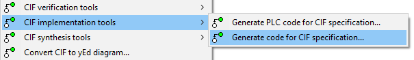
By default, you will get all internal variables at the output of the
SFunction, which is often too much. The Simulink Generation tab allows
precise definition of what output variables should be added, in this case all
variables in the controller automaton. (Input variables are never made
available from the CIF SFunction block, as they are already available in Simulink.)
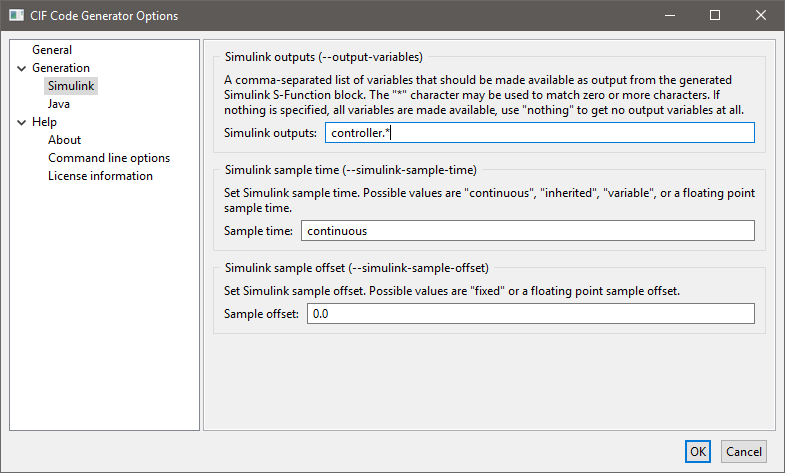
After selecting OK, the CIF model is translated to C code. Code generation
from the tank_ctrl.cif files results in two output files. The
tank_ctrl.c file contains the generated C source code. The
tank_ctrl_report.txt is a text file describing the data of the generated
SFunction code:
Input/output report of the tank_ctrl.cif SFunction.
During code generation, CIF variables are made available in the Simulink vectors.
This report lists the variables in each vector, along with their index number.
Modes
-----
controller 1
Continuous states
-----------------
time 1
Inputs
------
controller.V 1
Outputs
-------
controller.n 1The report shows which CIF variables are available at each vector. The
Inputs and Outputs are the most interesting. Here it shows that V is
the only input variable, n is the only output variable, and they are both
the first value in their vector. This is what you would expect for such
a small system. With bigger systems, the index numbers are much more useful
for making proper connections in Simulink.
And this concludes the CIF part of this example, next step is setting things up in Matlab/Simulink.
Simulation in Simulink
After starting Matlab, and moving to the correct directory, you get a display like:
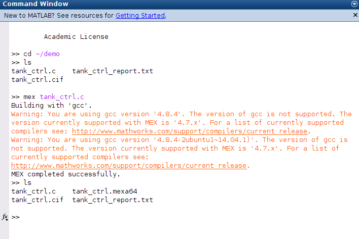
You can see the files present in the directory, as you would expect. In Matlab, the generated C code is compiled with the Matlab Mex compiler:
mex tank_ctrl.cHere, the compiler prints a warning about the wrong compiler version, this may be different at your system.
The result of the compilation is a tank_ctrl.mexa64 file at a 64 bit
system. If you use a 32 bit system, the filename extension is different.
The compiled CIF controller can be used in a Simulink System SFunction block, as shown below.

In the middle the equations are modeled. The output of the equations is V,
which is fed into the S-Function block with the CIF controller at the top.
The controller computes n which is an input for the equations.
At the bottom, a scope is attached that produces the following picture.
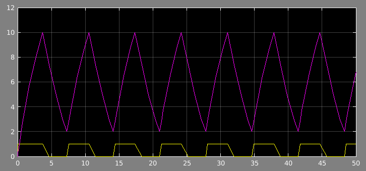
The volume fluctuates between 2 and 10, at the bottom is the control signal
n.
CIF PLC code generator
The CIF PLC code generator can be used to generate Programmable Logic Controller (PLC) code, for the implementation of CIF controllers on PLCs. The generated PLC code adheres to the IEC 61131-3 standard, a widely used international standard for PLC programming languages.
Starting the generator
The generator can be started in the following ways:
-
In Eclipse, right click a
.ciffile in the 'Project Explorer' tab or 'Package Explorer' tab and choose . -
In Eclipse, right click an open text editor for a
.ciffile and choose . -
Use the
cif2plctool in a ToolDef script. See the scripting documentation and tools overview page for details. -
Use the
cif2plccommand line tool.
Options
Besides the general application options, this application has the following options:
-
Input file: The absolute or relative local file system path to the input CIF specification.
-
Output file: The absolute or relative local file system path to the output file. Depending on the output type, this is either a file or a directory. The default depends on the output type as well.
-
PLC code output type: The PLC code output type specifies the type of output (essentially the file format) that should be generated.
-
PLC task name: The name of the PLC task to generate. If not specified, defaults to
PlcTask. -
PLC task cycle time: If periodic task scheduling is to be used, use this option to enable it, by setting the cycle time in milliseconds for the task to generate. The cycle time must be a positive integer number. Cycle times of over a minute may not work as expected. However, since such large cycle times are of little practical use, that should not be a problem. Disable this option to disable periodic task scheduling. This option defaults to periodic task scheduling with a cycle time of 10 milliseconds. Disabling periodic task scheduling is not supported for the TwinCAT output type.
-
PLC task priority: The scheduling priority of the task to generate. The priority must be in the range [0 .. 65535], where priority 0 is the highest priority, and priority 65535 is the lowest priority. The priority can be used for preemptive or non-preemptive scheduling. If not specified, the priority defaults to 20.
-
PLC project name: The name of the PLC project to generate. If not specified, defaults to
Untitled1. -
PLC configuration name: The name of the PLC configuration to generate. If not specified, defaults to
Untitled1. -
PLC resource name: The name of the PLC resource to generate. If not specified, defaults to
Untitled1. -
PLC number bits: The maximum number of bits supported by the PLC for representing numeric values. Use 64-bit if supported by the PLC, for full CIF compatibility, and the highest accuracy. If the PLC does not supported 64-bit integer and floating point numbers, set this option to 32-bit.
-
PLC maximum iterations: The maximum number of iterations of the main loop of the main program body, per execution of the main program body. Must be a positive number. May be set to infinite, to not impose a restriction. The default is set to at most 100 iterations. See the section on the program body for more information.
-
Formal function invocation (arguments based): Specifies for which functions to use formal invocation syntax in the generated PLC code. By default the formal syntax is used for none of the functions. For PLC implementations that don’t support the non-formal syntax, the formal syntax can be used for all functions, or only for functions with more than one argument.
-
Formal function invocation (function kind based): Specifies for which functions to use formal invocation syntax in the generated PLC code. By default the formal syntax is used only for all but the standard library/conversion functions. This can be changed to only the standard library/conversion functions, or to all functions.
-
Eliminate enumerations: Enable this option to eliminate enumerations before generating the actual PLC code, in case the PLC doesn’t support enumerations. Disable this option to keep enumerations in the generated PLC code. By default this option is disabled.
-
Simplify values: Enable this option to simplify values and inline constants during generation of the PLC code. The benefit is that static computations are evaluated, and for the result simpler PLC code is generated. This applies to both the original model as well as anything generated during the code generation, for instance as the result of linearization. Enabling the option may thus lead to simpler PLC code. However, the simplification itself may take quite some time. Furthermore, as constants are inlined, they are duplicated for each use. If a constant with a large value (such as a large literal array) is used multiple times, this can lead to significantly larger PLC code. By default this option is enabled.
-
Rename warnings: Enable this option to print warnings to the console when a PLC name is renamed due to a conflict with another PLC name, or disable it to omit the warnings. The option is disabled by default. See the section on names for more information.
Formal function invocation syntax (e.g. MIN(IN1:3, IN2:5)) is used in the
generated PLC code only for those functions that are included by both the
Formal function invocation (arguments based)
option and the
Formal function invocation (function kind based)
option. If either
of the options excludes the function, the non-formal function invocation syntax
(e.g. MIN(3, 5)) is used for that function. Note that for invocations of
function blocks, the generated PLC code always uses the formal syntax.
Furthermore, for certain standard library functions, only the non-formal syntax
is defined by the standard, and thus used in the generated PLC code.
Supported specifications
The CIF PLC code generator supports a subset of CIF specifications. The following restrictions apply:
-
Unrestricted events are not supported, as they can always be executed (are always enabled), and would lead to infinitely running PLC code. Detection of unrestricted events however, is incomplete. That is, for some unrestricted the code generation results in an error, while for other unrestricted events code is generated without any warnings or errors. See the Program body section for more information.
-
Specifications without automata are not supported.
-
Initialization predicates outside locations are not supported, except if it can be determined statically that they are trivially
true. -
State invariants in components are not supported, except if it can be determined statically that they are trivially
true. -
State/event exclusion invariants (in components as well as locations) are not supported. To allow state/event exclusion invariants to be used in the input, manually eliminate them first using the Eliminate state/event exclusion invariants CIF to CIF transformation.
-
Discrete variables with multiple initial values (including
any) are not supported. -
External user-defined functions are not supported.
-
Urgent locations are not supported.
-
Initialization predicates in locations that can not be statically evaluated are not supported.
-
State invariants in locations are not supported, except if it can be determined statically that they are trivially
true. -
Automata that do not have exactly one initial location are not supported.
-
Urgent edges are not supported.
-
User-defined functions without parameters are not supported.
-
Internal user-defined functions that contain a multi-assignment that assigns multiple (non-overlapping) parts of a single variable are not supported. For instance,
a[0], a[1] := 1, 2is not supported, as multiple parts (the first and second element) of arrayaare assigned in a single multi-assignment. This restriction applies only to multi-assignments in functions, not to multi-assignments on edges. -
Internal user-defined functions that contain a
continuestatement are not supported. -
Data types other than
bool,int(with or without range),real, enumerations, tuples, and arrays, are not supported. This applies to the data types of variables, parameters of functions, return types of functions, etc. -
String values are not supported.
-
Cast from
inttorealand casts that don’t change the type, are supported. All other casts are not supported. -
Sampling of distributions is not supported.
-
The use of the conjunction and disjunction binary operators on anything other than boolean values is not supported.
-
The use of the equality and inequality binary operators on anything other than boolean, integer, real, or enumeration values is not supported.
-
The use of the addition and subtraction binary operators on anything other than integer or real values is not supported.
-
The use of the element test and subset binary operators is not supported.
-
Projection on anything other than tuples and arrays is not supported. This applies to expressions as well as addressables (the left hand sides of assignments). For arrays, both 0-based indices (counting from the left) as well as negative indices (counting from the right) are supported.
-
Slicing is not supported.
-
Function calls on anything other than standard library functions and internal user-defined functions is not supported.
-
The
ceil,del,empty,floor,fmt,pop,round,scale,sign,size,acosh,asinh,atanh,cosh,sinh, andtanhstandard library functions are not supported. -
The distribution standard library functions are not supported.
-
Lists (except for arrays), sets, and dictionaries are not supported.
-
The use of functions as values is not supported. That is, functions may only be used in function calls, and may for instance not be stored in variables.
Preprocessing
The following CIF to CIF transformations are applied as preprocessing (in the given order), to increase the subset of CIF specifications that can be transformed:
-
Simplify values (if Simplify values option is enabled)
-
Eliminate constants (if Simplify values option is enabled)
After these preprocessing steps, the generator checks whether the specification is supported. It then applies the following additional CIF to CIF transformations:
-
Simplify values (if Simplify values option is enabled)
Standard compliance
The PLC code that is generated complies with the second edition (from 2003) of the IEC 61131-3 standard. The code does not use any vendor specific extensions, functions, etc.
For the TwinCAT output type, STRUCT
data type declarations have no ; character after the STRUCT data types,
to work around a bug in the TwinCAT parser. In that case the output is not
compliant with the IEC 61131-3 standard.
Generated PLC code
The bodies of the programs and functions in the generated PLC code use Structured Text as programming language. Structured Text is one of the programming languages that is part of the IEC 61131-1 standard.
The generated code contains a single program called MAIN. This program is
instantiated in a task, which is part of a resource, which in turn is part of
a configuration. The configuration is put in a project, but that is outside
the range of the IEC 61131-3 standard. Most implementations however, work with
projects. The effect of the project, configuration, resource, and task is
dependent on the output type. Besides a
program, the code generator also generates data types, functions, and global
variables.
For algebraic variables, functions are generated that are parametrized over the
state of the system. Similarly, functions are generated for the derivatives of
the continuous variables. For the discrete and continuous variables (including
variable time), a STRUCT data type named STATE is generated that
holds the entire state of the system (or more precisely, the
state of the CIF specification). For input variables,
an INPUTS global variables list/file is generated. For constants (if
Simplify values option is disabled), a CONSTS global variables list/file
is generated.
For invalid CIF specifications, the resulting code may not always behave as the
original CIF code. For instance, the ranges of integer types are ignored by the
code generator. Furthermore, mod by zero in CIF results in a runtime error,
while in the generated code it results in zero. Out of bound projection indices
of arrays may for instance have the effect that the closest existing element is
used instead, and the result may even be implementation dependent. There are
other such differences as well.
Little to no effort is put into generating readable code. That is, the generated is not meant to be inspected. The generated code is also not intended to be modified directly. Instead, the original CIF models should be modified, and from them new PLC code should be generated. Examples of non-readable code include the generated names, and code generated for expressions (which has way more parentheses than strictly necessary).
Names
The generated PLC code will contain names for functions, variables, locations of automata, etc. The absolute names of all objects are used. The names are influenced by the linearization algorithm. They are further influenced by the PLC code generator.
The code generator ensures unique names in the generated PLC code, taking into
account the reserved names (keywords, standard functions, etc) of the IEC
61131-3 standard and some of the common implementations of that standard. To
avoid reserved names, names are prefixed with prefixes that depend on the type
of object (for instance, dvar_ for discrete variables). Furthermore, it
takes into account that names in CIF are case sensitive, while they are case
insensitive in IEC 61131-3. The code generator computes a candidate name based
on these criteria.
If this results in duplicate names, renaming is performed. A common reason for
renaming is different locations (of the same automaton or of different
automata) that have the same name, but in different casing. For instance,
consider one location named WaitForTimeout and another named
WaitForTimeOut. After linearization, there is an enumeration with a literal
for each unique location name. The enumeration thus has at least two literals,
named WaitForTimeout and WaitForTimeOut. The candidate names for these
enumeration literals are elit_WaitForTimeout and elit_WaitForTimeOut.
However, they are identical except for casing. Thus, the first one that is
encountered during code generation gets the candidate name, and the second one
is renamed. This results in a warning like this:
WARNING: PLC variable "elit_WaitForTimeout" is renamed to "elit_WaitForTimeout2".Renaming may be needed to ensure valid functioning output. However, it may make it slightly more difficult to trace names in the generated PLC code back to the original CIF model. Also, in the PLC environment, when debugging the current values of variables may be shown. If enumeration literals are renamed, the renamed names may then be shown in the debugger. By default, the PLC code generator does not inform the user when renaming takes place. By enabling the Rename Warnings option, a warning will be printed to the console, each time a PLC name is renamed.
Program body
The body of the MAIN program consists of several parts. The MAIN
program is executed exactly once per cycle, by the PLC. The following parts are
present, and are executed in order:
-
Time and cycle time handling.
-
Initialization of the initial state, for the first cycle only.
-
Updating of the continuous variables for the time that has passed since the previous cycle, for all but the first cycle.
-
A loop that executes events for as long as they are possible.
The code automatically determines the cycle time that is used, in a manner that does not require any vendor specific extensions, functions, or data types. The generated code works for fixed cycle times (periodic task scheduling) as well as variable cycle times (non-periodic tasks).
During the first cycle, the variables of the state are initialized to their proper values. For subsequent cycles, the state resulting from the previous cycle is reused, where the values of the continuous variables are updated to account for the time that has passed since the beginning of the previous cycle. For details on the method used to update the values of the continuous variables, see the Accuracy over time section.
The loop at the end of the body evaluates the guard of each of the events of the CIF specification. If a guard holds, the corresponding update is performed. Code is generated for the events, or rather the edges, in the order that they occur in the linearized CIF specification. Linearization is performed in such a way, that the PLC code that is generated from it, has a correspondence to the simulator. Assuming the simulator is used to simulate by always automatically choosing the first transition that is enabled, the PLC code will choose that same transition. That is, for each iteration of the event loop, the code is executed for the first event with an enabled guard. Then, a new iteration of the loop is started, from the top, to ensure that the first enabled event is always executed, similar to simulation. If during an iteration of the loop none of the events is enabled, the loop terminates.
If at least one event was enabled, the loop is executed again. If during an iteration of the loop none of the edges was enabled, the loop terminates. This approach generally does not result in predictable execution times of the program body. That is, if a certain edge keeps being enabled, the loop is executed over an over again. In that case, the execution time of the body exceeds the fixed cycle time, and the controller is no longer guaranteed to work correctly. Even if the loop is only executed a finite number of times, the execution time of the body may exceed the fixed cycle time. One may consider monitoring the execution times to detect such issues.
Within the 'event loop', a counter is used to detect how often the loop is
repeated. After the loop is executed a 100 times, the loop is terminated, to
ensure that the body terminates in the case of events that are always possible.
In such a cases, variable loopsKilled is incremented by one, for debugging.
While by default the loop is terminated after 100 iterations, this maximum
number of iterations can be configured using the
PLC maximum iterations
option (Generator
category). The
option can also be set to infinite, to not impose a restriction, and never
terminate the loop due to too many iterations. See also the
Options section above.
Obviously, similar to the fact that the controller cannot guarantee its correct behavior if the execution time of a cycle exceeds the cycle time, the controller also cannot guarantee its correct behavior if the inputs from the external I/O change more rapidly than the cycle time. That is, if an input changes during a cycle, the change is not noticed until the next cycle. If an input changes during a cycle and changes back during that same cycle, the change is not noticed at all. Therefore, choosing an appropriate cycle time is essential for the correct functioning of the controller.
Accuracy over time
The generated code maintains the running time in seconds, by adding the cycle
time to current running time, on each cycle. Due to the finite binary
representation of real values, this results in loss of a accuracy over
prolonged periods of execution time. As such, the use of variable time in
CIF models is highly discouraged.
However, for a cycle time of one millisecond, while there may be loss of accuracy, time should keep increasing for at least several thousand years. After that, adding the cycle time may no longer increase the value of the variable, potentially resulting in unexpected execution behavior.
The continuous variables from the CIF specification are updated each cycle using the Euler method for integration. That is, each cycle the cycle time is multiplied by the derivative of the continuous variable in the state of the previous cycle. This value is added to the value of the continuous variable. Essentially, a linear approximation of the derivative is used, calculated using the state of the previous cycle.
The Euler method can be numerically unstable, can suffer from rounding errors due to the use finite binary representations of real values, and has some other issues as well. The effects are likely to be limited if linear continuous variable (continuous variables with constant derivatives) are used. Especially clocks (derivative +1 or -1) generally don’t suffer too much from these issues. However, even clocks may suffer from loss of accuracy over time. As such, clocks should not be used to measure over long periods of time. Instead they should be reset, rendering the past loss of accuracy irrelevant for any future measurements.
I/O coupling
For all variables in the state of the CIF specification, except for variable
time, PLC variables are generated with a %Q* address, to ensure they
can be used as output variables, and can potentially be coupled to output
ports. The state is maintained in a variable state0, a persistent local
variable of the MAIN program.
For all input variables of the CIF specification, a PLC variable is generated
with a %I* addresses, to ensure they can be used as input variables, and
can potentially be coupled to input ports. These variables are generated in a
global variables list/file named INPUTS.
The actual coupling to hardware addresses is something that is left to the implementation of the PLC programming environment.
PLC output type
The PLC code generator can generate its output in multiple forms (file formats) depending on the output type. The output type can be configured using the PLC code output type option ( Generator category). The following output types are currently available:
-
PLCopen XML (default)
-
IEC 61131-3
PLCopen XML is an
XML-based file format
standardized by the PLCopen organization, intended for the exchange of complete
projects of PLC code, even across different tools and vendors. The PLCopen
XML files generated by the PLC code generator are compliant with version 2.01
of the PLCopen XML standard. By default, if no output file is specified, it
defaults to the input file path, where the .cif file extension is removed
(if present), and a .plcopen.xml file extension is added.
Output in IEC 61131-3 syntax generates multiple files. By default, if no output
directory is specified, it defaults to the input file path, where the .cif
file extension is removed (if present), and a _plc directory extension is
added. The MAIN program gets a .plcprog file extension, functions get
a .plcfunc file extension, type declarations get a .plctype file
extension, and the configuration gets a .plccfg file extension. The
PLC project name and PLC resource name options have no effect for this
output type.
TwinCAT is a complete
IDE
for the
development and testing of PLC controllers. Using the TwinCAT PLC output type,
the generated PLC code can be written to the native file formats of the TwinCAT
IDE. By default, if no output directory is specified, it defaults to the input
file path, where the .cif file extension is removed (if present), and a
_twincat directory extension is added. See the
TwinCAT PLC output page for further details.
TwinCAT PLC output
TwinCAT is a complete IDE for the development and testing of PLC controllers. Using the TwinCAT PLC output type, the generated PLC code can be written to the native file formats of the TwinCAT IDE. This allows for more tight integration and smoother development cycles than using the PLCopen XML output type.
We currently only provide official support for version 3.1 of TwinCAT.
TwinCAT system modes
The TwinCAT software IDE is built on Microsoft Visual Studio. TwinCAT also supplies a utility to monitor and control the TwinCAT System Service, via an icon in the system tray, part in the Windows taskbar. The icon shows the mode (or status) of the TwinCAT system:
-
 Inactive Mode
 -
 Stop Mode
 -
 Config Mode
 -
 Run Mode
 -
 Exception Mode
In the Inactive Mode, the TwinCAT System Service is not running. Restart Windows or manually activate the TwinCAT System Service and related services.
The Stop Mode is of little use, so switch to the Config Mode instead. In the Config Mode, the system (the PLC) can be configured. In the Run Mode, the system (the PLC) can be used to control the hardware. If a runtime exception occurs in Run Mode, the Exception Mode becomes active.
Within Visual Studio, the mode is also shown as an icon in the bottom right corner of the IDE:
-
Stop Mode
-
Config Mode
-
Run Mode
-
/
 Free Run Mode (alternating icons)
 -
Exception Mode
If the system is only equipped with a soft PLC, and the TwinCAT environment is set up to target the local system, both icons should indicate a consistent status. This page assumes this situation.
Changing modes
To change to Config Mode or restart Config Mode from the system tray:
-
Right click the system tray icon and choose .
To change to Config Mode or restart Config Mode from Visual Studio:
-
Click . Alternatively, click the appropriate toolbar item (
 ).
). -
A dialog pops up with the question Restart TwinCAT System in Config Mode. Click OK or press ENTER.
-
A dialog pops up with the question Load I/O Devices. Click Yes or press ENTER.
-
A dialog pops up with the question Activate Free Run. Click Yes or press ENTER.
To change to Run Mode or restart Run Mode from the system tray:
-
Make sure the hardware is powered up.
-
Right click the system tray icon and choose .
To change to Run Mode or restart Run Mode from Visual Studio:
-
Make sure the hardware is powered up.
-
Click . Alternatively, click the appropriate toolbar item (
 ).
). -
A dialog pops up with the question Restart TwinCAT System in Run Mode. Click OK or press ENTER.
In general it is recommended to switch modes via Visual Studio instead of via the system tray icon.
Generated output
The CIF PLC code generator can generate code into an existing TwinCAT Visual
Studio solution, with a TwinCAT XAE project that contains a TwinCAT Standard
PLC project. The directory that contains the solution must have the same name
(except for the file extension) as the solution file (.sln file). The
TwinCAT XAE project (both the directory and the .tsproj file) in the
solution should have the same name as well. The TwinCAT XAE project should
contain a TwinCAT Standard PLC project. This project may be given any name,
and this name can be configured using the
PLC project name
option
(Generator
category). However, in order to be able to import I/O
mappings it is highly recommended to always use the default name suggested by
TwinCAT (Untitled1) for TwinCAT Default PLC projects.
The project should already contain a task. This task can be given any name,
and this name can be configured using the
PLC task name
option
(Generator
category). By default, TwinCAT Default PLC projects have
a task named PlcTask. This name is the default for the
PLC task name
option as well. The cycle time and priority of the
task are automatically updated by the PLC code generator, depending on the
values provided for the options of the generator. The code generator also
ensures that the MAIN program is instantiated/scheduled on the task.
All POU (functions, programs, etc), DUT (data types), and GVL
(global variable lists) code files that are present in the TwinCAT Default PLC
project are removed, from both the project and from disk, by the PLC code
generator. The newly generated code files are (over)written, and the project is
updated to include and compile only the newly generated files.
The PLC configuration name and PLC resource name options have no effect on the TwinCAT output.
TwinCAT usage
Follow these steps to create a solution and project in TwinCAT, generate PLC code in it, and use the PLC code to control the hardware:
-
Start TwinCAT (Visual Studio) by right clicking on the TwinCAT system tray icon and choosing TwinCAT XAE (VS 2010).
-
Create a new TwinCAT XAE project:
-
Click .
-
In the New Project window, TwinCAT XAE Project (XML format) should already be selected. If not, first select TwinCAT Project on the left (from the list of Installed Templates), and then select TwinCAT XAE Project (XML format).
-
Choose a project name and enter it in the Name box at the bottom of the dialog.
-
Make sure the Solution name is exactly the same, and that the Create directory for solution option is enabled.
-
For Location, select the directory in which the directory for the solution should be created. This is usually the directory that contains the script and/or source files you will be using to generate the PLC code.
-
To figure out the directory that contains the ToolDef script, make sure that the Properties view is visible in Eclipse. Select the ToolDef script in the 'Project Explorer' tab or 'Package Explorer' tab, and look for the location property.
-
-
Click OK to create the project.
-
-
Scan the available hardware:
-
Make sure the hardware is powered up.
-
Make sure the Config Mode is enabled, by switching to it if it is not the current mode.
-
In the project, under I/O, right click the Devices item and choose Scan. Alternatively, select the I/O item and click the appropriate toolbar item (
 ).
). -
A dialog pops up with the warning HINT: Not all types of devices can be found automatically. Click OK or press ENTER.
-
A dialog pops up where you have to choose the I/O device to scan. Normally, if you have only one I/O device, it should already be selected. Click OK or press ENTER.
-
A dialog pops up with the question Scan for boxes. Click Yes or press ENTER.
-
A dialog pops up with the question Activate Free Run. Click Yes or press ENTER.
-
-
Create a new TwinCAT PLC project:
-
Right click the PLC item in the project, and choose Add New Item….
-
In the Add New Item dialog, Standard PLC project should already be selected.
-
Keep the name
Untitled1in the Name box at the bottom of the dialog. -
Also don’t change the Location of the project.
-
Click Add to add the PLC project.
-
-
Save the entire solution by clicking .
-
Generate PLC code. If using a script, wait for the execution of the script to finish (the status indicated as part of the title of the console should change from
runningtoFINISHED). -
Switch back to TwinCAT (Microsoft Visual Studio).
-
When a File Modification Detected window pops up for the project, click Reload to reload the updated project that was written by the CIF tooling.
-
Build the project by clicking .
-
Load the I/O mappings:
-
In the project, under I/O, right click Mappings, and choose Import Mapping Infos….
-
Select the mappings file for your hardware, and click Open.
-
If the import succeeds, you should see an Untitled1 Instance - … item under the Mappings item.
-
-
Activate the configuration:
-
Click . Alternatively, click the appropriate toolbar item (
 ).
). -
A dialog pops up with the question Activate Configuration (Old Configurations will be overwritten!). Click OK or press ENTER.
-
A dialog pops up with the question Restart TwinCAT System in Run Mode. Click OK or press ENTER.
-
-
Start the PLC:
-
Click . Alternatively, click the appropriate toolbar item (
 ).
). -
A dialog pops up with the question Application Port_851 does not exist on the device. Do you want to create it and proceed with download?. Click Yes or press ENTER.
-
Click . Alternatively, click the appropriate toolbar item (
 ).
).
-
-
The PLC is now running, and you can use the system.
To stop the PLC:
-
Click . Alternatively, click the appropriate toolbar item (
 ).
). -
Click . Alternatively, click the appropriate toolbar item (
 ). This step is optional, and can usually be
skipped.
). This step is optional, and can usually be
skipped.
To reset the PLC and start the 'simulation' from the beginning, with the same code and the same configuration:
-
Make sure the hardware is powered up.
-
Load the I/O mappings, if the Untitled1 Instance - … item under the Mappings item is no longer present:
-
In the project, under I/O, right click Mappings, and choose Import Mapping Infos….
-
Select the mappings file for your hardware, and click Open.
-
If the import succeeds, you should see an Untitled1 Instance - … item under the Mappings item.
-
-
Reactivate the configuration:
-
Click . Alternatively, click the appropriate toolbar item (
). -
A dialog pops up with the question Activate Configuration (Old Configurations will be overwritten!). Click OK or press ENTER.
-
A dialog pops up with the question Restart TwinCAT System in Run Mode. Click OK or press ENTER.
-
-
Start the PLC:
-
Click . Alternatively, click the appropriate toolbar item (
). -
A dialog pops up with the question Application Port_851 does not exist on the device. Do you want to create it and proceed with download?. Click Yes or press ENTER.
-
Click . Alternatively, click the appropriate toolbar item (
).
-
-
The PLC is now running, and you can use the system.
Whenever you change a CIF source file, regenerate a supervisor, change a hardware mapping, etc, you need to regenerate the PLC code as well. Follow these steps:
-
Make sure the Config Mode is enabled, by switching to it if it is not the current mode.
-
Save the entire solution in TwinCAT by clicking .
-
Regenerate PLC code from Eclipse. If using a script, wait for the execution of the script to finish (the status indicated as part of the title of the console should change from
runningtoFINISHED). -
Switch back to TwinCAT (Microsoft Visual Studio).
-
For all File has been changed outside the environment. Reload the new file? questions, click Yes or press ENTER. See the Frequently Asked Questions (FAQ) for instructions on how to disable some of these questions.
-
When a File Modification Detected window pops up for the project, click Reload to reload the updated project that was written by the CIF tooling.
-
Clean the project by clicking .
-
Rebuild the project by clicking .
-
Make sure the hardware is powered up.
-
Reload the I/O mappings:
-
In the project, under I/O, right click Mappings, and choose Import Mapping Infos….
-
Select the mappings file for your hardware, and click Open.
-
If the import succeeds, you should see an Untitled1 Instance - … item under the Mappings item.
-
-
Activate the configuration:
-
Click . Alternatively, click the appropriate toolbar item (
). -
A dialog pops up with the question Activate Configuration (Old Configurations will be overwritten!). Click OK or press ENTER.
-
A dialog pops up with the question Restart TwinCAT System in Run Mode. Click OK or press ENTER.
-
-
Start the PLC:
-
Click . Alternatively, click the appropriate toolbar item (
). -
A dialog pops up with the question Application Port_851 does not exist on the device. Do you want to create it and proceed with download?. Click btn:Yes[] or press ENTER.
-
Click . Alternatively, click the appropriate toolbar item (
).
-
-
The PLC is now running, and you can use the system.
Frequently Asked Questions (FAQ)
-
Question: Is there something that can be done about the large number of File has been changed outside the environment… prompts?
Answer: Yes. Click to show the Options dialog. On the left, select . Then, on the right, enable the Detect when file is changed outside the environment and Auto-load changes, if saved options.
-
Question: Why doesn’t importing the I/O mappings have any effect?
Answer: Make sure the TwinCAT Standard PLC project is named
Untitled1, and try again. Also, make sure you’ve built the solution before you try to import the I/O mappings. -
Question: I get a dialog with the warning Device '…' needs a sync master (at least one variable linked to a task variable). What should I do?
Answer: You probably forgot to load an I/O mapping.
-
Question: Why does opening the MAIN program take so long in Run Mode?
Answer: As the generated code becomes larger, it can take a long time for TwinCAT to set up the environment for inline monitoring of the MAIN program. To disable inline monitoring, click to show the Options dialog. On the left, select . Then, on the right, switch to the Monitoring tab. Disable the Enable inline monitoring option.
-
Question: TwinCAT hangs for long periods of time, before crashing and automatically being restarted by Windows. What should I do?
Answer: If the generated code is too large, TwinCAT may not be able to handle it. In such cases, reduce the size of the generated code, by reducing the size of the CIF model for which you are generating the code.
-
Question: I get an error stating 'Reading file failed. […]'. What should I do?
Answer: The generated code is too large for TwinCAT to handle. See also the answer to the previous question.
Miscellaneous tools
CIF to CIF transformer
The CIF to CIF transformer can be used to syntactically transform CIF specifications to similar CIF specifications, which behave in the same manner (are semantically equivalent), but are expressed using different language constructs. For example, the CIF to CIF transformation that eliminates constants, replaces all uses of constants by their values, and removes the constants from the specification.
These reusable transformations are primarily used to increase the subset of CIF specifications that can be transformed or processed. Usually, there is no need to apply the CIF to CIF transformations manually. Transformations that work on subsets of the CIF language, automatically apply the necessary CIF to CIF transformations as a preprocessing step, to increase the translatable subset.
The CIF to CIF transformer can also be used as a pretty printer.
Starting the transformation
The transformation can be started from Eclipse in the following ways:
-
Right click a
.ciffile in the 'Project Explorer' tab or 'Package Explorer' tab and choose . -
Right click an open text editor for a
.ciffile and choose . -
Use the
cif2ciftool in a ToolDef script. See the scripting documentation and tools overview page for details. -
Use the
cif2cifcommand line tool.
Options
Besides the general application options, this application has the following options:
-
Input file path: The absolute or relative local file system path to the input CIF specification.
-
Output file path: The absolute or relative local file system path to the output CIF specification. If not specified, the output file path defaults to the input file path, where the
.ciffile extension is removed (if present), and a.transformed.ciffile extension is added. -
Transformations: The CIF to CIF transformations to apply. The transformations are applied in the chosen order. Transformations may be applied multiple times. By default, no transformations are applied, essentially making the CIF to CIF transformer a pretty printer.
In the option dialog, the available transformations are shown. To add a transformation, double click it, or select it and click the Add button below the list of available transformations. To remove a transformation, double click on it in the list of chosen transformations, or select it in that list and click the Remove button.
At the command line, specify comma separated transformation names, in the order they should be applied. The names to use are listed below, in the Available transformations section.
Transformation descriptions
The pages describing the available transformations all use the same format. They have the following sections:
-
Introduction: describes the transformation in a few sentences.
-
Supported specifications: describes the subset of CIF specifications to which the transformation can be applied.
-
Preprocessing: specifies the CIF to CIF transformations that are automatically applied as preprocessing, or the CIF to CIF transformations that can be manually applied as preprocessing, to increase the subset of CIF specifications that can be transformed by the transformation.
-
Implementation details: further specifies what the transformation does, how it does it, and what the result of the transformation is. Most transformations also show one or more examples.
-
Renaming: explains if and when renaming may be performed by the transformation.
-
Size considerations: describes whether the transformation reduces or increases the size of the specification. If the specification may increase in size, an estimate of the order of increase is given (linear, exponential, etc). Note that the size is not the file size, but rather the number of objects used to represent the specification (the number of automata, locations, edges, guards, binary operators, etc).
-
Optimality: describes why the transformation result may not be optimal, if applicable. May also explain how to eliminate certain concepts that may be introduced as the result of the transformation.
Available transformations
A whole collection of CIF to CIF transformations is available. The available transformations are listed below, with a link to the information about the transformation, and the name to use for that transformation on the command line.
-
Add default initial values (
add-default-init-values) -
Eliminate algebraic variables (
elim-alg-vars) -
Eliminate automata to string casts (
elim-aut-casts) -
Eliminate component definition/instantiation (
elim-comp-def-inst) -
Eliminate constants (
elim-consts) -
Eliminate enumerations (
elim-enums) -
Eliminate equations (
elim-equations) -
Eliminate groups (
elim-groups) -
Eliminate
ifupdates (elim-if-updates) -
Eliminate the use of locations in expressions (
elim-locs-in-exprs) -
Eliminate monitors (
elim-monitors) -
Eliminate automaton
selfreferences (elim-self) -
Eliminate state/event exclusion invariants (
elim-state-event-excl-invs) -
Eliminate
tauevent (elim-tau-event) -
Eliminate tuple field projections (
elim-tuple-field-projs) -
Eliminate type declarations (
elim-type-decls) -
Lift events (
lift-events) -
Linearize (merge) (
linearize-merge) -
Linearize (product) (
linearize-product) -
Merge enumerations (
merge-enums) -
Push print file declarations into print declarations (
print-file-into-decls) -
Remove CIF/SVG declarations (
remove-cif-svg-decls) -
Remove I/O declarations (
remove-io-decls) -
Remove print declarations (
remove-print-decls) -
Remove position information (
remove-pos-info) -
Remove requirements (
remove-reqs) -
Simplify others (
simplify-others) -
Simplify values (
simplify-values) -
Simplify values (optimized) (
simplify-values-optimized) -
Simplify values (no references) (
simplify-values-no-refs) -
Simplify values (no references, optimized) (
simplify-values-no-refs-optimized) -
Push SVG file declarations into other CIF/SVG declarations (
svg-file-into-decls) -
Convert
switchexpressions toifexpressions (switches-to-ifs)
Pretty printer
If no transformations are applied by the CIF to CIF transformer, the input CIF specification is just read from the input file, validated, and written to the output file. This can be useful, as it essentially turns the CIF to CIF transformer into a CIF pretty printer.
As a side effect of reading the input file and validating it, the model may change slightly. In fact, this occurs not only for the CIF to CIF transformer but for all tools, as they all read input files and validate them, before continuing with their actual task. Examples of such changes include the elimination of imports, the loss of comments, and the evaluation of tuple projection indices.
Add default initial values
This CIF to CIF transformation adds the default initial values to variables that are not given an explicit initial value. This includes discrete and continuous variables, as well as local variables of functions.
Supported specifications
This transformation supports a subset of CIF specifications. The following restrictions apply:
-
Component definitions and component instantiations are not supported.
Preprocessing
No preprocessing is currently performed by this CIF to CIF transformation. To increase the subset of specifications that can be transformed, apply the following CIF to CIF transformations (in the given order):
Implementation details
The default values for all types are simple values. The only exception are
function types, for which a new function is introduced. This new functions
returns the default value for the return type of the function. If multiple
default values for the same function type are needed, the newly introduced
function is reused. The functions are named _f, _f2, _f3, etc.
For instance, the following specification:
automaton x:
disc int x, y = 5;
disc func bool (int) f;
location;
endis transformed to the following specification:
func bool _f(int p0):
return false;
end
automaton x:
disc int x = 0, y = 5;
disc func bool (int) f = _f;
location;
endRenaming
If the names of the functions that are introduced, conflict with already
existing declarations, they are renamed. For instance, if _f2 is already in
use, _f22, _f23, etc, are used instead. If renaming takes place, a
warning is printed to the console.
Size considerations
Since values are added, this transformation increases the size of the specification. For an array of 400 elements, with an array of 300 integers each, the default initial value consists of 1,200 integers. Add such an initial value can significantly increase the size of the model.
Optimality
The default values for all types are as primitive as they can be, and can usually not be simplified any further. It may however be possible that functions are introduced for the default values of function types, while such a function already existed in the original specification.
Convert switch expressions to if expressions
This CIF to CIF transformation converts switch expressions to if
expressions.
Supported specifications
This transformation supports all CIF specifications.
Preprocessing
n/a
Implementation details
All switch expressions are replaced by if expressions. For instance,
consider the following CIF specification:
alg int y = ...
alg real x = switch y:
case 1: 1.0
case 2: 4.0
case 3: 9.0
else 0.0
end;
alg real z = switch y:
else 1.0
end;
automaton a:
alg string v = switch self:
case l1: "first"
case l2: "second"
end;
location l1:
initial;
edge tau goto l2;
location l2;
endThis is transformed to the following CIF specification:
alg int y = ...
alg real x = if y = 1: 1.0
elif y = 2: 4.0
elif y = 3: 9.0
else 0.0
end;
alg real z = 1.0;
automaton a:
alg string v = if l1: "first"
else "second"
end;
location l1:
initial;
edge tau goto l2;
location l2;
endFor algebraic variable z, there is only one case (the else), so no
if expression is generated. This optimization means that the control value
(y in this case) is lost.
For algebraic variable v in automaton a, the switch expression uses
an automaton self reference. The cases list the possible locations of the
automaton, and the switch expression maps them to string values. Since for
if expressions the else part is mandatory, the last case of the
switch is converted to the else of the if expression.
Renaming
n/a
Size considerations
The created if expression is usually larger than the original switch
expression, as the control value is duplicated for each if and elif
part, where it is compared to the case values. For switch expressions
with only one case or else, no if expression is generated, and the
expression becomes smaller.
Optimality
This transformation transforms switch expressions to if expressions,
leading to if expressions with if and elif guards that may not be
optimal. To simplify the result, apply additional CIF to CIF transformations,
such as Simplify values.
Eliminate algebraic variables
This CIF to CIF transformation eliminates algebraic variables and their equations.
See also: Eliminate equations.
Supported specifications
This transformation supports a subset of CIF specifications. The following restrictions apply:
-
Component definitions and component instantiations are not supported.
-
Automaton
selfreferences are not supported.
Preprocessing
No preprocessing is currently performed by this CIF to CIF transformation. To increase the subset of specifications that can be transformed, apply the following CIF to CIF transformations (in the given order):
Implementation details
For each algebraic variable with a single equation in a component or automaton, all uses of the variable (for instance in guards, invariants, etc) are replaced by the value of the variable (the right hand side of its equation). For algebraic variables with equations specified in the locations of an automaton, an 'if' expression is created. This 'if' expression uses the locations of the automaton as guards, and the right hand sides of the equations as values for each of the alternatives. The last alternative is an 'else', and thus has no guard. If the automaton has only one location, generation of the 'if' expression is suppressed.
The algebraic variables and their equations are removed.
For instance, the following specification:
alg bool b1 = true;
alg bool b2;
equation b2 = false;
automaton aut:
alg int a;
location l1:
equation a = 1;
location l2:
equation a = 2;
end
invariant b1 or b2 or p.a > 0;is transformed to the following specification:
automaton aut:
location l1;
location l2;
end
invariant true or false or if p.l1: 1 else 2 end > 0;Renaming
n/a
Size considerations
Since algebraic variables are shortcuts for expressions, eliminating them could result in an increase of the size of the specification. Algebraic variables may be defined in terms of other algebraic variables. Therefore, in the worst case, the increase is exponential.
Optimality
For an assignment x := 1 + y, where y is an algebraic variable that is
eliminated, and where y has value 5, the resulting assignment is
x := 1 + 5. The result is not simplified any further. To further simplify
the result, apply additional CIF to CIF transformations, such as
Simplify values.
This transformation introduces 'if' expressions for algebraic variables that have an equation per location, for automata with at least two locations. The guards of such 'if' expressions refer to the locations of the automata. To eliminate such location references, apply the Eliminate the use of locations in expressions CIF to CIF transformation.
Eliminate automata to string casts
This CIF to CIF transformation eliminates casts of automata to strings.
Supported specifications
This transformation supports a subset of CIF specifications. The following restrictions apply:
-
Component definitions and component instantiations are not supported.
Preprocessing
No preprocessing is currently performed by this CIF to CIF transformation. To increase the subset of specifications that can be transformed, apply the following CIF to CIF transformations (in the given order):
Implementation details
All casts of automata to strings, using either implicit automaton self
references or explicit automata references, are eliminated. If the referred
automaton has only a single location, the cast is replaced by a string literal
with the name of that location. If the automaton has multiple locations, the
cast is replaced by an if expression, using the locations of the automaton
as guards, and string literals containing the location names as values. For
nameless locations the string literal "*" is used.
For instance, consider the following CIF specification:
automaton a:
alg string x = <string>self;
location:
initial;
end
automaton b:
alg string x = <string>self;
location l1:
initial;
location l2:
endThis is transformed to the following CIF specification:
automaton a:
alg string x = "*";
location:
initial;
end
automaton b:
alg string x = if l1: "l1"
elif l2: "l2"
else "l3"
end;
location l1:
initial;
location l2;
location l3;
endRenaming
n/a
Size considerations
The created if expressions are usually larger than the original cast
expressions. The increase is linear in terms of the number of locations times
the number of casts.
Optimality
This transformation introduces 'if' expressions for automaton to string casts, for automata with at least two locations. The guards of such 'if' expressions refer to the locations of the automata. To eliminate such location references, apply the Eliminate the use of locations in expressions CIF to CIF transformation.
Eliminate component definition/instantiation
This CIF to CIF transformation eliminates all component definitions and instantiations, by actually instantiating the component definitions.
Supported specifications
This transformation supports all CIF specifications.
Preprocessing
n/a
Implementation details
This transformation operates in three phases:
-
Phase 1: Find the component definitions without any component definitions and/or component instantiations in them.
-
Phase 2: Instantiate the component definitions found in phase 1, by putting the body of the definition in the place of the instantiation, in a component named after the component instantiation. Also removes the component definitions that were just instantiated, and introduces new local algebraic variables for the algebraic parameters.
-
Phase 3: Replace uses of component, event, and location parameters by the actual arguments provided for the instantiation.
For instance, the following specification:
group def P(alg int x):
invariant x > 0;
end
p1: P(1);
alg int y = 2;
p2: P(y);is transformed to the following specification:
group p1:
alg int x = 1;
invariant x > 0;
end
alg int y = 2;
group p2:
alg int x = y;
invariant x > 0;
endAbsolute references may be needed to express the results of this transformation. For instance:
const int x = 5;
group def X():
invariant x = 5;
end
group a:
x: X();
endis transformed to the following specification:
const int x = 5;
group a:
group x:
invariant .x = 5;
end
endNote how the invariant in component a.x can not refer to constant x
directly, as x refers to component a.x in that context. Therefore, the
scope absolute reference .x is used instead.
Renaming
n/a
Size considerations
Since component definitions are shortcuts for components, eliminating them could result in an increase of the size of the specification.
Optimality
n/a
Eliminate constants
This CIF to CIF transformation eliminates constants.
Supported specifications
This transformation supports a subset of CIF specifications. The following restrictions apply:
-
Component definitions and component instantiations are not supported.
Preprocessing
No preprocessing is currently performed by this CIF to CIF transformation. To increase the subset of specifications that can be transformed, apply the following CIF to CIF transformations (in the given order):
Implementation details
All uses of constants (for instance in guards, invariants, etc), are replaced by their values. The constants themselves are removed. For instance, the following specification:
const int x = 1;
const int z = y;
const int y = x + 1;
invariant x + y + z > 0;is transformed to the following specification:
invariant 1 + 2 + 2 > 0;Renaming
n/a
Size considerations
Since constants are shortcuts for values, eliminating them could result in an increase of the size of the specification. Constants may be defined in terms of other constants. Therefore, in the worst case, the increase is exponential.
Optimality
For an assignment x := 1 + y, where y is a constant that is eliminated,
and where y has value 5, the resulting assignment is x := 1 + 5.
The result is not simplified any further. To further simplify the result, apply
additional CIF to CIF transformations, such as
Simplify values.
Eliminate enumerations
This CIF to CIF transformation eliminates enumerations.
See also: Merge enumerations.
Supported specifications
This transformation supports a subset of CIF specifications. The following restrictions apply:
-
Component definitions and component instantiations are not supported.
Preprocessing
To increase the subset of specifications that can be transformed, apply the following CIF to CIF transformations (in the given order) prior to using this transformation:
Implementation details
Enumerations, which are used as types, are replaced by integer types, with
range [0 .. n-1], where n is the number of literals of the enumeration.
Enumeration literals, which are used as values, are replaced by integer values.
If the used enumeration literal is the nth literal in the corresponding
enumeration (declaration), then the integer value is n - 1. That is, the
integer value is the 0-based index of the enumeration literal into the literals
of the enumeration declaration.
All enumeration declarations are removed.
For instance, the following specification:
group x:
enum EX = A, B;
const EX x = A;
end
group y:
enum EY = B, A;
const EY y = A;
endis transformed to the following specification:
group x:
const int[0..1] x = 0;
end
group y:
const int[0..1] y = 1;
endRenaming
This transformation itself does not perform any renaming.
If enumeration literals are renamed, this may influence value equality for compatible enumerations (enumerations with the same number of literals, with the same names, in the same order). Therefore, either apply this transformation before applying other transformations that perform renaming on enumeration literals (such as the Eliminate groups CIF to CIF transformation), or otherwise ensure that renaming does not result in an invalid specification.
Size considerations
Integer types and integer values are not larger than enumerations and their literals. Therefore, this transformation does not increase the size of the specification. In fact, it may even be smaller.
Optimality
n/a
Eliminate equations
This CIF to CIF transformation eliminates equations for algebraic variables and derivatives of continuous variables. Note that it does not eliminate the variables themselves.
See also: Eliminate algebraic variables.
Supported specifications
This transformation supports a subset of CIF specifications. The following restrictions apply:
-
Component definitions and component instantiations are not supported.
-
Automaton
selfreferences are not supported.
Preprocessing
No preprocessing is currently performed by this CIF to CIF transformation. To increase the subset of specifications that can be transformed, apply the following CIF to CIF transformations (in the given order):
Implementation details
For algebraic variables with a single equation in a component or automaton, the value of the variable (the right hand side of the equation) is moved to the declaration of the algebraic variable. For algebraic variables with equations specified in the locations of an automaton, an 'if' expression is created. This 'if' expression uses the locations of the automaton as guards, and the right hand sides of the equations as values for each of the alternatives. The last alternative is an 'else', and thus has no guard. The single right hand side, or the 'if' expression, is put directly in the declaration of the algebraic variable. If the automaton has only one location, generation of the 'if' expression is suppressed.
The derivatives of continuous variables are transformed in a similar way. The derivative ends up in the declaration of the continuous variable.
All equations are removed from components (including automata) and locations.
For instance, the following specification:
alg bool b1 = true;
cont x;
equation x' = 1.0;
automaton p:
alg int a;
location l1:
equation a = 1;
location l2:
equation a = 2;
endis transformed to the following specification:
alg bool b1 = true;
cont x der 1.0;
automaton p:
alg int a = if l1: 1
else 2
end;
location l1;
location l2;
endRenaming
n/a
Size considerations
The right hand sides of the equations are simply moved. This does not influence the size of the specification. For equations specified in the locations of an automaton, an 'if' expression is created. This increases the size of the specification. The increase however, is linear in the number of equations.
Optimality
This transformation introduces 'if' expressions for algebraic variables and derivatives of continuous variables that have an equation per location of an automaton, for automata with at least two locations. The guards of such 'if' expressions refer to the locations of the automata. To eliminate such location references, apply the Eliminate the use of locations in expressions CIF to CIF transformation.
Eliminate groups
This CIF to CIF transformation flattens the component structure of a specification, by eliminating all groups. That is, after this transformation, all automata will be at the top level, directly in the specification.
Supported specifications
This transformation supports a subset of CIF specifications. The following restrictions apply:
-
Component definitions and component instantiations are not supported.
Furthermore, this transformation does not guarantee the correct result for specification with enumerations. See also the Renaming section below.
Preprocessing
To increase the subset of specifications that can be transformed, apply the following CIF to CIF transformations (in the given order) prior to using this transformation:
The following CIF to CIF transformations are automatically applied as preprocessing (in the given order), to increase the subset of CIF specifications that can be transformed:
Implementation details
All declarations, invariants, initialization predicates, marker predicates, and equations from the groups are lifted to the top level of the specification. The automata are lifted to the top level of the specification as well. Subsequently, the groups are removed.
In order to be able to track the origin of automata and declarations, they are
named after their absolute names. For a group x, with a group
y, with a constant z, the absolute name of the constant is x.y.z.
The constant is lifted to the top level of the specification, and named
x_y_z.
For instance, this specification:
group a:
const int x = 5;
invariant x > 4;
end
group p:
automaton q:
event e;
location;
end
endis transformed to the following specification:
const int a_x = 5;
invariant a_x > 4;
automaton p_q:
event e;
location;
endRenaming
Since declarations of the specification are merged with the declarations of the
groups and with automata, renaming may be necessary to ensure uniquely
named declarations. For instance, for a group x, with a group
y, with a constant z, the absolute name of the constant is x.y.z.
The constant is lifted to the top level of the specification, and renamed to
x_y_z. However, if the specification already contains a declaration of
another constant, automaton, etc named x_y_z, then the lifted constant is
renamed to x_y_z2 instead. If that name is also already in use, it is
renamed to x_y_z3, etc.
Whenever renaming takes place, a warning will be printed to the console.
Enumeration literals that are part of lifted enumeration declarations, are not renamed to their absolute names. To understand why this is necessary, consider:
group x:
enum E = A, B;
end
automaton y:
enum E = A, B;
location:
initial;
end
invariant x.A = y.A;Here, group x and automaton y both have an enumeration E with
enumeration literals A and B. The invariant of the specification
compares the literals of the two different enumerations. This is allowed, since
the enumerations are compatible (they have the same enumeration literals,
with the same names, in the same order). If we were to rename the enumeration
literals to absolute names as we lift them to the top level of the
specification, the result would be:
enum x_E = x_A, x_B;
automaton y:
enum E = A, B;
location:
initial;
end
invariant x_A = y.A;Which would no longer be a valid specification, as enumerations x_E and
y.E are no longer compatible (they have enumeration literals with different
names). Since we leave the names of the enumeration literals as they are, the
result of the transformation is:
enum x_E = A, B;
automaton y:
enum E = A, B;
location:
initial;
end
invariant A = y.A;which is still a correct specification, and has the same meaning as the original specification.
Now assume the following specification:
group x:
enum E = A, B;
end
group y:
enum E = A, B;
end
invariant x.A = y.A;Here, the two enumerations are both in groups. If we lift them, we have two enumerations, with the same literals, which is not a valid CIF specification. As such, renaming can not be avoided, and the result of the transformation will be:
enum x_E = A, B;
enum y_E = A2, B2;
invariant A = A2;This result is an invalid CIF specification. Whenever an enumeration literal is renamed, a warning is printed to the console, informing of the possibility that the resulting specification is invalid. As such, it is highly recommended to avoid such situations, and eliminate the enumerations prior to the elimination of the groups.
Size considerations
The groups are removed. Other objects are lifted, which essentially means they are moved. The size of the specification does not increase.
Optimality
n/a
Eliminate if updates
This CIF to CIF transformation eliminates 'if' updates on edges.
Supported specifications
This transformation supports a subset of CIF specifications. The following restrictions apply:
-
Multi-assignments and partial variable assignments are not supported. That is, the left hand sides of the assignments on edges (the addressables) must be single variables without projections.
Preprocessing
No preprocessing, to increase the subset of CIF specifications that can be transformed, is currently performed by this CIF to CIF transformation.
Implementation details
This transformation ensures that each variable that is assigned, gets a single explicit assignment. Simply put, the 'if' update structure is replicated by an 'if' expression. For instance, the following edge updates:
if g:
if g2:
x := 5
else
y := 6
end
end,
z := 7are transformed to the following edge updates:
x := if g:
if g2:
5
else
x
end
else
x
end,
y := if g:
if g2:
y
else
6
end
else
y
end,
z := 7Observe how variables x and y are assigned inside two if updates.
These if updates are replicated by two if expressions.
Since for if expressions the else part is not optional, dummy
x := x assignments are sometimes performed in cases where the original
specification would not have assigned variable x at all. That is, variables
may be assigned their old values, resulting in superfluous assignments.
Renaming
n/a
Size considerations
The 'if' structure may be replicated for multiple variables, which may result in an increase of the specification size. The increase amount is influenced by the size of the guard expressions, and the number of levels of nesting 'if' updates.
Optimality
The superfluous assignments (see the Implementation details section above), are obviously not optimal. The language however requires them.
Eliminate the use of locations in expressions
This CIF to CIF transformation eliminates the use of locations in expressions (such as guards, invariants, and equations), by introducing location pointer variables for automata, and using them instead.
Supported specifications
This transformation supports a subset of CIF specifications. The following restrictions apply:
-
Component definitions and component instantiations are not supported.
Preprocessing
No preprocessing is currently performed by this CIF to CIF transformation. To increase the subset of specifications that can be transformed, apply the following CIF to CIF transformations (in the given order):
Implementation details
For each automaton for which a location is used (referred to) in an expression (such as a guard, invariant, or equation), a location pointer variable is introduced, with as value the current location of the automaton. The values for such a new variables are part of a newly created enumeration that has a value (an enumeration literal) for each location of the automaton.
To initialize the new location pointer variable, the variable itself is
initialized to any (meaning any value in its domain), and initialization
predicates are added to all locations that could potentially be initial
locations. For automata with exactly one initial state, the initial value
of the location pointer variable is set directly, instead of using
initialization predicates.
All edges in the automaton that change the current location of that automaton, get an additional assignment to update the location pointer variable.
All uses of the locations of the automaton in expressions (that is, all location reference expressions) are changed to equality binary expressions for the location pointer variable and the enumeration literal corresponding to the location.
For instance, the following specification:
automaton x:
event e;
alg bool a = l1;
location l1:
initial;
edge e goto l2;
location l2:
edge e;
endis transformed to the following specification:
automaton x:
event e;
alg bool a = LP_x = LOC_l1;
disc LOCS_x LP_x = LOC_l1;
enum LOCS_x = LOC_l1, LOC_l2;
location l1:
initial;
edge e do LP_x := LOC_l2 goto l2;
location l2:
edge e;
endLocation pointer variable LP_x is added. It is initialized directly in the
declaration, since there is exactly one initial location in this automaton.
Enumeration LOCS_x is created to represent the possible values of the
location pointer variable. Enumerations literals LOC_l1 and LOC_l2
represent locations l1 and l2, respectively.
The edge from location l1 to location l2 is extended with an update
to the location pointer. The self loop in location l2 is not extended, as
the location does not change.
Renaming
If the names of the location pointer variables that are introduced, conflict
with already existing declarations, they are renamed. For instance, if LP_x
is already in use, LP_x2, LP_x3, etc, are used instead. Similarly,
renaming is performed for enumerations, and enumeration literals that conflict
with already existing declarations. If renaming takes place, a warning is
printed to the console.
Size considerations
The number of added location pointer variables is linear in the number of automata. The number of added initialization predicates for the location pointer variables is linear in the number of possible initial locations. The number of added enumerations is linear in the number of automata. The number of added enumeration literals is linear in the number of locations. The number of added updates is linear in the number of edges. The number of added equality binary expressions is linear in the number of location references.
Optimality
This transformation introduces enumerations for the possible values of the location pointer variables. To eliminate the enumerations, apply the Eliminate enumerations CIF to CIF transformation.
Eliminate monitors
This CIF to CIF transformation eliminates monitor events.
Supported specifications
This transformation supports a subset of CIF specifications. The following restrictions apply:
-
Component definitions and component instantiations are not supported.
Preprocessing
No preprocessing is currently performed by this CIF to CIF transformation. To increase the subset of specifications that can be transformed, apply the following CIF to CIF transformations (in the given order):
Implementation details
For each monitor event in an automaton, additional self loops are added as needed, to make sure the automaton doesn’t disable the monitor event. Furthermore, all monitors are removed from all automata.
The self loop edges created by this transformation have no communication
(no !..., no ?...), no urgency (no now), and no updates
(no do ...).
For instance, for the following locations and edges, for monitor event e:
location l1:
edge e goto l2;
edge f when x = 2 goto l3;
location l2:
edge e when x = 1 goto l3;
edge e when x = 2 goto l1;
location l3;the result after this transformation is:
location l1:
edge e goto l2;
edge f when x = 2 goto l3;
location l2:
edge e when x = 1 goto l3;
edge e when x = 2 goto l1;
edge e when not(x = 1 or x = 2);
location l3:
edge e;In location l1, monitor event e is always enabled (no guard implies
a true guard), and thus no additional self loop is needed. In location
l2, event e is only enabled if x has either value 1 or value
2. A self loop is added for all other cases, to ensure the event is always
enabled. In location l3, the event is never enabled (no edges, which
essentially means guard false). A self loop is added, to ensure the event
is always enabled.
Event f is not a monitor event, and is thus not affected by this
transformation.
Renaming
n/a
Size considerations
Since self loop edges may be added by this transformation, the size of the specification may increase.
Optimality
For an edge with guard x = 1, a self loop with guard not (x = 1) may
be generated by this transformation. The guard could be simplified to
x != 1. However, this transformation does not simplify guards. To further
simplify the result, apply additional CIF to CIF transformations, such as
Simplify values.
Eliminate automaton self references
This CIF to CIF transformation replaces implicit automaton self references
by explicit automaton references.
Supported specifications
This transformation supports a subset of CIF specifications. The following restrictions apply:
-
Component definitions and component instantiations are not supported.
Preprocessing
No preprocessing is currently performed by this CIF to CIF transformation. To increase the subset of specifications that can be transformed, apply the following CIF to CIF transformations (in the given order):
Implementation details
All implicit automaton self references are replaced by explicit automaton
references. For instance, consider the following CIF specification:
automaton a:
alg string x = <string>self;
location:
initial;
endThis is transformed to the following CIF specification:
automaton a:
alg string x = <string>a;
location:
initial;
endRenaming
n/a
Size considerations
Since both references are single expression nodes, this transformation does not increase the size of the specification.
Optimality
n/a
Eliminate state/event exclusion invariants
This CIF to CIF transformation eliminates state/event exclusion invariants. It replaces them with automata with self loops.
Supported specifications
This transformation supports a subset of CIF specifications. The following restrictions apply:
-
Component definitions and component instantiations are not supported.
Preprocessing
No preprocessing is currently performed by this CIF to CIF transformation. To increase the subset of specifications that can be transformed, apply the following CIF to CIF transformations (in the given order):
Implementation details
All state/event exclusion invariants are removed from the specification.
They are replaced with automata with self loops. Per component, the state/event exclusion invariants of the component (the top level scope of the specification, groups, automata), as well as those of its locations (only for automata), are partitioned per supervisory kind. Per such partition, an automaton is created.
The automaton is put along side the component (for groups and automata), as
sibling. For invariants in the top level scope of the specification, the new
automaton is put in the top level scope of the specification. The new automaton
gets the same name as the component that contained the invariants as prefix,
with some postfixes. For invariants at the top level scope of the
specification, an empty prefix is used. The first postfix is indicates the
supervisory kind of the invariants of the partition: Plant,
Requirement, Supervisor, or empty for regular/kindless invariants.
The second postfix is StateEvtExcls. So, for an automaton Abc with
some plant invariants, an automaton AbcPlantStateEvtExcls is created. The
name may conflict with existing automata or other declarations, in which case
it is renamed.
The automata that are created inherit the supervisory kind of the state/event exclusion invariants in the partition for which the automaton is created. The automata have a single nameless location, that is both initial and marked.
For each state/event exclusion invariant in the partition, and self loop edge is created per event. The condition predicates of the invariants are used as guard, possible after some manipulation.
For state/event exclusion invariants of the locations of automata, the
condition predicate is made conditional on the location. However, this is only
done for automata with at least two locations, as conditioning on an always
active location is of little use. For a location loc, and a state/event
exclusion invariant invariant evt needs x = 1, predicate x = 1 is
changed to loc => x = 1.
For state/event exclusion invariants that indicate when an event is to be
disallowed/disabled, the condition predicate is inverted. The inversion is
performed after the condition predicate is made condition on the location, if
applicable. For instance, for a state/event exclusion invariant
invariant x != 1 disables evt in a location loc, the condition
predicate x != 1 is first made conditional on the location. This results in
loc => x != 1. The condition predicate is then inverted to
not(loc => x != 1), which is then used as guard.
The alphabets of the automata are left implicit.
Consider the following example CIF specification:
plant automaton aut:
controllable e1, e2, e3;
disc int[0..10] x;
requirement invariant e1 needs x < 10;
requirement invariant x = 0 disables {e1, e2};
location:
initial;
requirement invariant x = 0 disables e3;
edge e1 do x := x + 1;
edge e2 do x := x - 1;
edge e3 do x := 0;
endIt is transformed to the following CIF specification:
plant automaton aut:
controllable e1, e2, e3;
disc int[0..10] x;
location:
initial;
edge e1 do x := x + 1;
edge e2 do x := x - 1;
edge e3 do x := 0;
end
requirement automaton autRequirementStateEvtExcls:
location:
initial;
marked;
edge aut.e1 when aut.x < 10, not(aut.x = 0);
edge aut.e2 when not(aut.x = 0);
edge aut.e3 when not(aut.x = 0);
endRenaming
New automata are created. If the desired name for an automaton is already in
use for some other automaton or declaration, the new automaton is given a
different name. For instance, if an automaton is to be named
ControllerStateEvtExcls and that name is already in use, it will be named
ControllerStateEvtExcls2. If that name is also already in use, it will be
named ControllerStateEvtExcls3, etc.
Size considerations
The constant amount of additional objects are created (e.g. an automaton, a
location, a true initialization predicate, etc). At most one automaton is
created per state/event exclusion invariant. As such, the size increase is
linear in the number of state/event exclusion invariants.
Optimality
For state/event exclusion invariants that are defined in locations of automata with more than one location, this transformation makes their predicates conditional on those locations. To eliminate such location references, apply the Eliminate the use of locations in expressions CIF to CIF transformation.
This transformation generate boolean implication and inversion predicates. These are not simplified. To simply them, apply the the Simplify values CIF to CIF transformation.
Eliminate tau event
This CIF to CIF transformation eliminates the tau event.
Supported specifications
This transformation supports all CIF specifications.
Preprocessing
n/a
Implementation details
This transformation introduces new events for the tau event, one per
automaton where a tau event is used. The new events are named tau_ (if
that name is not already in use).
If the alphabet is explicit specified, it is extended as well.
The new events are neither controllable nor uncontrollable, and don’t have a data type.
For instance, the following specification:
automaton p:
event e;
location l1:
initial;
edge when true goto l2;
location l2:
edge e, tau goto l1;
endis transformed to the following specification:
automaton p:
event e;
event tau_;
location l1:
initial;
edge tau_ when true goto l2;
location l2:
edge e, tau_ goto l1;
endRenaming
The newly introduced tau_ events are renamed to tau_2, tau_3, etc,
if they conflict with other declarations with the same name, that already
exist in the automata. If renaming is needed, a warning is printed to the
console.
Size considerations
New events may be added, the alphabet may be extended, and an explicit event may be added to edges. Therefore, the size of the specification may increase.
Optimality
n/a
Eliminate tuple field projections
This CIF to CIF transformation eliminates tuple field projections by replacing them with tuple index projections.
Supported specifications
This transformation supports all CIF specifications.
Preprocessing
n/a
Implementation details
Obtaining the value of a field of a tuple is called tuple projection. There are two ways to project a tuple. That is, there are two ways to indicate from which field to obtain the value. The first way is to use the name of the field, the second way is to use the 0-based index of the field into the fields of the tuple’s type. For instance:
const tuple(int a; real b) t = (1, 2.0);
const int x = t[a];
const int y = t[0];Here, both constants x and y have value 1, obtained from field
a of the tuple value of constant t.
This transformation replaces tuple field projections (using the name of the field), by tuple index projections (using the 0-based index of the field). For instance, for the example above, the result of this transformation is:
const tuple(int a; real b) t = (1, 2.0);
const int x = t[0];
const int y = t[0];Renaming
n/a
Size considerations
Since both field references and integer values are single expression nodes, this transformation does not increase the size of the specification.
Optimality
n/a
Eliminate type declarations
This CIF to CIF transformation eliminates type declarations.
Supported specifications
This transformation supports a subset of CIF specifications. The following restrictions apply:
-
Component definitions and component instantiations are not supported.
Preprocessing
No preprocessing is currently performed by this CIF to CIF transformation. To increase the subset of specifications that can be transformed, apply the following CIF to CIF transformations (in the given order):
Implementation details
All uses of type declarations (in types of variables, types of other type declarations, etc), are replaced by the types of those type declarations. The type declarations themselves are removed. For instance, the following specification:
type t = int;
type u = v;
type v = tuple(t a, b);
const t x = 1;
const u y = (2, 3);
const v z = (4, 5);is transformed to the following specification:
const int x = 1;
const tuple(int a, b) y = (2, 3);
const tuple(int a, b) z = (4, 5);Renaming
n/a
Size considerations
Since type declarations are shortcuts for types, eliminating them could result in an increase of the size of the specification. Type declarations may be defined in terms of other type declarations. Therefore, in the worst case, the increase is exponential.
Optimality
n/a
Lift events
This CIF to CIF transformation lifts event declarations to the top level of the specification.
Supported specifications
This transformation supports a subset of CIF specifications. The following restrictions apply:
-
Component definitions and component instantiations are not supported.
-
Groups are not supported.
Preprocessing
No preprocessing is currently performed by this CIF to CIF transformation. To increase the subset of specifications that can be transformed, apply the following CIF to CIF transformations (in the given order):
Implementation details
All events declared in the automata, are lifted to the top level of the specification.
In order to be able to track the origin of the events, they are named after
their absolute names. For a group x, with a group y, with an
event e, the absolute name of the event is x.y.e. The event is lifted
to the top level of the specification, and named x_y_e.
For instance, this specification:
event e;
automaton a:
event e;
location;
end
group b:
automaton c:
event e;
location;
end
endis transformed to the following specification:
event e;
event a_e;
event b_c_e;
automaton a:
location;
end
group b:
automaton c:
location;
end
endRenaming
Since events of the automata are merged with the declarations of the
specification, renaming may be necessary to ensure uniquely named declarations.
For instance, for a group x, with a group y, with an event
e, the absolute name of the event is x.y.e. The event is lifted to the
top level of the specification, and renamed to x_y_e. However, if the
specification already contains a declaration of a constant, automaton, other
event, etc, named x_y_e, then the lifted event is renamed to x_y_e2
instead. If that name is also already in use, it is renamed to x_y_e3, etc.
Whenever renaming takes place, a warning is be printed to the console.
Size considerations
Events are lifted, which essentially means they are moved. The size of the specification does not increase.
Optimality
n/a
Linearize (merge)
This CIF to CIF transformation performs process-algebraic linearization, thereby eliminating parallel composition and event synchronization.
Supported specifications
This transformation supports a subset of CIF specifications. The following restrictions apply:
-
Specifications without automata are not supported.
Preprocessing
The following CIF to CIF transformations are applied as preprocessing (in the given order), to increase the subset of CIF specifications that can be transformed:
Implementation details
A location pointer variable is introduced for each original automaton, and the
use of locations in expressions is eliminated. This is mostly similar to what
the Eliminate the use of locations in expressions CIF to CIF transformation does,
except that for instance location pointer variables are added for all automata.
For nameless locations, name X is used.
One new automaton, named M, is created. If all original automata have
the same supervisory kind, the new automaton gets this kind as well. Otherwise,
it gets no supervisory kind. The alphabet of this new automaton is the union of
alphabets of the original automata, including the events that are used to
send or receive in any of the automata.
All declarations from the original automata are moved to the new automaton.
They are renamed based on their absolute names. That is, for an automaton a
with a constant c, the absolute name of the constant is a.c and the
moved constant will be named a_c. Enumeration literals are not given
absolute names, and keep their original names
if possible.
One location, named L, is added. This location is both initial and marked.
All initialization and marker predicates from all the original automata
(including ones from locations) are merged together. They are put in the new
automaton, and restrict the initialization and marker predicates of location
L.
The invariants of the original automata (including ones from locations) are merged together in a similar way as the initialization and marker predicates. The supervisory kinds of the invariants are made explicit, to ensure that the original supervisory kinds inherited from automata are preserved.
For the tau event, a self loop is created per original tau edge. For
all other events, the edges are merged, resulting in a single self loop for
each non-tau event. By creating single edges per non-tau event,
non-deterministic choice may be
eliminated, ensuring that the model size of the resulting specification is
near-linear compared to the model
size of the original specification.
Monitors are taken into account when merging the guards of the edges, resulting in simpler guard predicates. Communication is eliminated altogether, and events no longer have data types after linearization. For edges with receives, the 'received value' is replaced (in the updates) by the 'send value'.
For instance, the following specification:
event e;
plant automaton p:
disc int x = 1;
location l1:
initial;
edge e when x = 1 do x := 2 goto l2;
location l2:
edge e when x = 2 do x := 1 goto l1;
end
plant automaton q:
location l1:
initial;
edge tau goto l2;
location l2:
edge e goto l1;
endis transformed to the following specification:
event e;
enum E = l1, l2;
plant automaton M:
alphabet e;
disc int p_x = 1;
disc E p = l1;
disc E q = l1;
initial p = l1 and true or p = l2 and false,
q = l1 and true or q = l2 and false;
marked p = l1 and false or p = l2 and false,
q = l1 and false or q = l2 and false;
location L:
initial;
marked;
edge e when (p = l1 and p_x = 1 or p = l2 and p_x = 2) and
(q = l1 and false or q = l2 and true)
do if p = l1 and p_x = 1: p_x := 2, p := l2
elif p = l2 and p_x = 2: p_x := 1, p := l1
end,
q := l1;
edge tau when q = l1 do q := l2;
endWe see that an enumeration E is added, with literals for all the locations
of the original automata. We also see that plant automata p and q are
linearized to plant automaton M. Two location pointers, p and q,
named after the original automata, are added. The variables are moved. The
initialization and marker predicates are linearized. We have one location
L, which is initial and marked. For event e, the guards and updates are
linearized into a single self loop. Location pointer updates are incorporated
as well. For event tau, the single original edge is simply included as a
self loop.
If the original automata have non-determinism, this choice is eliminated as
part of this transformation. Non-determinism can be present due to multiple
outgoing edges for a single location, for the same event (excluding the
tau event), with overlapping guards. Another cause of non-determinism is
multiple senders or receivers that are enabled at the same time, for the same
channel. In the resulting specification, the first possible transition is
always taken, similar to how the simulator chooses, assuming the simulator is
configured to always automatically choose the
first transition. Linearization eliminates some of the
non-determinism in this case, essentially choosing a specific trace through
the state space. To ensure the same choices are made, events and automata are
sorted in the same order for linearization and simulation.
For instance, the following specification:
automaton p:
event e;
disc int x = 0;
location:
edge e when x < 5 do x := x + 1;
edge e when x > 3 do x := x - 1;
endis transformed to the following specification:
enum E = X;
automaton M:
alphabet p_e;
event p_e;
disc int p_x = 0;
disc E p in any;
initial p = X and false;
marked p = X and false;
location L:
initial;
marked;
edge p_e when p = X and (p_x < 5 or p_x > 3)
do if p = X and p_x < 5: p_x := p_x + 1
elif p = X and p_x > 3: p_x := p_x - 1
end;
endHere, we see that the edge for event e with guard x < 5 and update
x := x + 1 is chosen to take precedence over the edge with guard x > 3
with update x := x - 1. This choice is based on the original specification,
where the edge with guard x < 5 is listed before the edge with guard
x > 3.
Related to this, are dummy updates, which are added to ensure that the correct updates are taken. For instance, the following specification:
automaton p:
event e;
disc int x = 0;
location:
edge e when x >= 3;
edge e when x < 3 do x := x + 1;
endis transformed to the following specification:
enum E = X;
automaton M:
alphabet p_e;
event p_e;
disc int p_x = 0;
disc E p in any;
initial p = X and false;
marked p = X and false;
location L:
initial;
marked;
edge p_e when p = X and (p_x >= 3 or p_x < 3)
do if p = X and p_x >= 3: p := X
elif p = X and p_x < 3: p_x := p_x + 1
end;
endHere, the edge with guard x >= 3 takes precedence over the edge with guard
x < 3. To ensure that no updates are performed when the edge with guard
x >= 3 is chosen, a dummy update is added (reassigning the location pointer
variable the value it already has). If this update were to be omitted, the
update of the other edge would instead be executed, which is undesirable.
If code generation is performed on a linearized version of the specification, it may be a good idea to ensure the same order is used and the same choices are made, both in the generated code and in simulation. Assuming simulation was performed by always automatically choosing the first transition, this should correspond to the output of linearization. The linearized edges are in the same order as the transitions are calculated by the simulator. This is ensured by sorting events and automata in the same order for linearization and simulation. Also, as the Non-determinism section above explains, if non-determinism is eliminated, it is done in a way that preserves that order.
Code should thus be generated in the order of the linearized edges resulting from linearization. Each time the code for an edge is executed, the code should start from the top, to ensure always the first enabled transition is chosen.
If the original automata contain urgent locations and/or urgent edges, a
discrete boolean variable u is added to the linearized automaton.
Initially, it’s value is true, and it must always remain so
(plant invariant u;). We add self loops (event tau), with as guard the
urgent locations and guards of urgent edges, such that the edge can be taken if
the system is in an urgent location, or an urgent edge is enabled (guard wise).
However, these edges update u to false, which violates the target
location invariant, meaning we can never take these edges in a transition.
Since the edge is also urgent, it means that if the edge is enabled guard wise,
time may not progress, thus ensuring the urgency behavior of the original
urgent locations and edges.
For instance, the following specification:
automaton p:
event e;
location l1:
initial;
urgent;
edge e when true goto l2;
location l2:
edge e when 1 = 1 now goto l1;
endis transformed to the following specification:
enum E = l1, l2;
automaton M:
alphabet p_e;
event p_e;
disc E p = l1;
disc bool u = true;
initial p = l1 and true or p = l2 and false;
marked p = l1 and false or p = l2 and false;
plant invariant u;
location L:
initial;
marked;
edge p_e when p = l1 and true or p = l2 and 1 = 1
do if p = l1 and true: p := l2
elif p = l2 and 1 = 1: p := l1
end;
edge when p = l1 or p = l2 and 1 = 1 now do u := false;
endSo, if p (the location pointer variable for original automaton p) is
equal to l1 (the enumeration literal for original location l1), then
the guard of the new urgent edge is enabled, and time may not progress.
Similarly, if p is equal to l2 and the guard 1 = 1 of the original
urgent edge is enabled, the guard of the new urgent edge is enabled, and time
may not progress. This correctly reflects the urgency conditions of the
original specification.
To ensure that no additional event transitions are possible, the new urgent
edge can never be taken, as it would update u to false, which violates
plant invariant u.
The following specification:
event tuple(int a, b) e;
automaton s:
location:
edge e!(1, 2);
end
automaton r:
disc int x;
location:
edge e? do x := ?[a];
endis transformed to the following specification:
event e;
enum E = X;
automaton M:
alphabet e;
disc E s in any;
disc int r_x;
disc E r in any;
initial s = X and false,
r = X and false;
marked s = X and false,
r = X and false;
location L:
initial;
marked;
edge e when s = X and true and (r = X and true) do r_x := (1, 2)[0];
endObserve how event e no longer has a data type, and the communication (send
and receive) have been eliminated. In the assignment x := ?[a], received
value ? has been replaced by send value (1, 2). Since tuple values
don’t have field names, the right hand side (1, 2)[a] has been replaced
by (1, 2)[0], using the Eliminate tuple field projections CIF to
CIF transformation.
Since channel communication is completely eliminated, and channels become regular events after this transformation, it is no longer possible to merge additional senders/receivers with the linearized specification. If you wish to merge another specification with additional communication partners, first perform the merging, and then the linearization.
Renaming
Since declarations are moved/merged, and new names are introduced, renaming may
be necessary to ensure unique names within a single scope. In order to reduce
the amount of renaming for the enumeration literals introduced for the
locations of the original automata, all enumerations are merged together into a
single enumeration in the specification, with name E.
If renaming is performed, a warning is printed to the console.
Size considerations
Declarations are moved, so they don’t increase the size of the specification.
The addition of location variables increases the size of the specification, but this is linear in the number of automata and the number of locations.
Assignment are added for the updates to the location pointers. The increase is linear in the number of edges. The additional dummy updates that are added are linear in the number of edges as well.
A single self loop is added for each non-tau event. This does increase the
size of the specification. The guards are simply combined using boolean
operators, and the increase is therefore linear in the number of guards.
Similarly, updates are combined using 'if' updates, and the increase is also
linear.
For original edges with multiple events however, the guards and updates are duplicated for each event. The duplication is linear in the number of events on those edges.
Since tau edges are essentially just moved, they don’t increase the size
of the specification. That is, their size is linear in the number of original
tau edges.
The initialization and marker predicates, as well as the invariants are moved. They remain linear in size related to the number of original predicates. The predicates for the locations are also made conditional on the values of the location pointer variable. This size increase is linear in the number of original locations. Predicates are combined using boolean operators, leading to a size increase that is linear in the number of original predicates.
If a single received value is used multiple times in the updates of a single edge, the send value is duplicated for each of those uses. As such, the size increase is linear in the number of uses of the received value.
If multiple senders and multiple receivers (individual send/receive edges, not whole automata) are present for a certain event, then the received value is expanded to all the potential send values, with the conditions under which they are used as send value (using an 'if' expression). As such, the received value are expanded into expressions that are linear in the number of senders. If we have only a single sender or a single receiver, this is linear. If we have multiple of both, this becomes quadratic (number of senders times number of receivers).
For urgency, an additional variable and invariant are added. This is a constant increase in size. A self loop is added as well. This self loop duplicates the guards of urgent edges. It also includes predicates for the urgent locations. The size of this edge is linear in the number of urgent locations, and the guards of the urgent edges.
From the above, it should be clear that while the specification may increase in size, it is mostly linear. Practically, the size of the linearized specification is usually linear compared to the size of the input specification.
Optimality
As should be clear from the examples above, this transformation does not try to generate optimized expressions. In fact, often almost all generated expressions can easily be simplified. To further simplify the result, apply additional CIF to CIF transformations, such as Simplify values.
Currently, no effort is made by this transformation to reduce for instance the number of dummy assignments, or the number of replacements of tuple field projections by tuple index projections.
Linearize (product)
This CIF to CIF transformation performs process-algebraic linearization, thereby eliminating parallel composition and event synchronization.
Supported specifications
This transformation supports a subset of CIF specifications. The following restrictions apply:
-
Specifications without automata are not supported.
Preprocessing
The following CIF to CIF transformations are applied as preprocessing (in the given order), to increase the subset of CIF specifications that can be transformed:
Implementation details
A location pointer variable is introduced for each original automaton, and the
use of locations in expressions is eliminated. This is mostly similar to what
the Eliminate the use of locations in expressions CIF to CIF transformation does,
except that for instance location pointer variables are added for all automata.
For nameless locations, name X is used.
One new automaton, named M, is created. If all original automata have
the same supervisory kind, the new automaton gets this kind as well. Otherwise,
it gets no supervisory kind. The alphabet of this new automaton is the union of
alphabets of the original automata, including the events that are used to
send or receive in any of the automata.
All declarations from the original automata are moved to the new automaton.
They are renamed based on their absolute names. That is, for an automaton a
with a constant c, the absolute name of the constant is a.c and the
moved constant will be named a_c. Enumeration literals are not given
absolute names, and keep their original names
if possible.
One location, named L, is added. This location is both initial and marked.
All initialization and marker predicates from all the original automata
(including ones from locations) are merged together. They are put in the new
automaton, and restrict the initialization and marker predicates of location
L.
The invariants of the original automata (including ones from locations) are merged together in a similar way as the initialization and marker predicates. The supervisory kinds of the invariants are made explicit, to ensure that the original supervisory kinds inherited from automata are preserved.
For the tau event, a self loop is created per original tau edge. For
all other events, the
Cartesian product
of all
edges is created, combining the edges in all possible combinations. This
results in self loops for all non-tau events, where the combination of all
self loops maintains all non-deterministic choices of the original
specification. Worst case, the model size of the resulting specification
compared to the model size of the original specification
could blow up exponentially.
Monitors are taken into account when merging the guards of the edges, resulting in simpler guard predicates. Communication is eliminated altogether, and events no longer have data types after linearization. For edges with receives, the 'received value' is replaced (in the updates) by the 'send value'.
For instance, the following specification:
event e;
plant automaton p:
disc int x = 1;
location l1:
initial;
edge e when x = 1 do x := 2 goto l2;
location l2:
edge e when x = 2 do x := 1 goto l1;
end
plant automaton q:
location l1:
initial;
edge tau goto l2;
location l2:
edge e goto l1;
endis transformed to the following specification:
event e;
enum E = l1, l2;
plant automaton M:
alphabet e;
disc int p_x = 1;
disc E p = l1;
disc E q = l1;
initial p = l1 and true or p = l2 and false,
q = l1 and true or q = l2 and false;
marked p = l1 and false or p = l2 and false,
q = l1 and false or q = l2 and false;
location L:
initial;
marked;
edge e when p = l1 and p_x = 1 and q = l2
do p_x := 2, p := l2, q := l1;
edge e when p = l2 and p_x = 2 and q = l2
do p_x := 1, p := l1, q := l1;
edge tau when q = l1 do q := l2;
endWe see that an enumeration E is added, with literals for all the locations
of the original automata. We also see that plant automata p and q are
linearized to plant automaton M. Two location pointers, p and q,
named after the original automata, are added. The variables are moved. The
initialization and marker predicates are linearized. We have one location
L, which is initial and marked. For event e, two self loop edges are
added, as automaton p has two edges for e and automaton q has one
edge for e and 2 * 1 is 2. For the self loop edges, the guards and
updates are combined. Location pointer updates are incorporated as well. For
event tau, the single original edge is simply included as a self loop.
If the original automata have non-determinism, this choice is maintained as
part of this transformation. Non-determinism can be present due to multiple
outgoing edges for a single location, for the same event (excluding the
tau event), with overlapping guards. Another cause of non-determinism is
multiple senders or receivers that are enabled at the same time, for the same
channel. In the resulting specification, all possible combinations are
included as self loops. For a specification with 4 sender automata with two
send edges each (8 send edges in total) and 5 receiver automata with two
receive edges each (10 receive edges in total) for event e, and also 6
automata with two edges each that synchronize over that event (12
synchronization edges in total), the number of possible combinations for
communication with synchronization is 8 * 10 * 12, which is 960
possible combinations.
For instance, the following specification:
event e;
automaton p:
disc int x = 0;
location:
edge e when x < 5 do x := x + 1;
edge e when x > 3 do x := x - 1;
end
automaton q:
disc int y = 0;
location:
edge e when y < 5 do y := y + 1;
edge e when y > 3 do y := y - 1;
edge e when y = 4 do y := y - 1;
endis transformed to the following specification:
event e;
enum E = X;
automaton M:
alphabet e;
disc int p_x = 0;
disc E p in any;
disc int q_y = 0;
disc E q in any;
initial p = X and false,
q = X and false;
marked p = X and false,
q = X and false;
location L:
initial;
marked;
edge e when p = X and p_x < 5 and q = X and q_y < 5
do p_x := p_x + 1, q_y := q_y + 1;
edge e when p = X and p_x < 5 and q = X and q_y > 3
do p_x := p_x + 1, q_y := q_y - 1;
edge e when p = X and p_x < 5 and q = X and q_y = 4
do p_x := p_x + 1, q_y := q_y - 1;
edge e when p = X and p_x > 3 and q = X and q_y < 5
do p_x := p_x - 1, q_y := q_y + 1;
edge e when p = X and p_x > 3 and q = X and q_y > 3
do p_x := p_x - 1, q_y := q_y - 1;
edge e when p = X and p_x > 3 and q = X and q_y = 4
do p_x := p_x - 1, q_y := q_y - 1;
endHere, we see that for event e, automaton p has two edges and automaton
q has three edges. The linearization result has six edges.
If code generation is performed on a linearized version of the specification, it may be a good idea to ensure the same order is used and the same choices are made, both in the generated code and in simulation. Assuming simulation was performed by always automatically choosing the first transition, this should correspond to the output of linearization. The linearized edges are in the same order as the transitions are calculated by the simulator. This is ensured by sorting events and automata in the same order for linearization and simulation.
Code should thus be generated in the order of the linearized edges resulting from linearization. Each time the code for an edge is executed, the code should start from the top, to ensure always the first enabled transition is chosen.
If the original automata contain urgent locations and/or urgent edges, a
discrete boolean variable u is added to the linearized automaton.
Initially, it’s value is true, and it must always remain so
(plant invariant u;). We add self loops (event tau), with as guard the
urgent locations and guards of urgent edges, such that the edge can be taken if
the system is in an urgent location, or an urgent edge is enabled (guard wise).
However, these edges update u to false, which violates the target
location invariant, meaning we can never take these edges in a transition.
Since the edge is also urgent, it means that if the edge is enabled guard wise,
time may not progress, thus ensuring the urgency behavior of the original
urgent locations and edges.
For instance, the following specification:
automaton p:
event e;
location l1:
initial;
urgent;
edge e when true goto l2;
location l2:
edge e when 1 = 1 now goto l1;
endis transformed to the following specification:
enum E = l1, l2;
automaton M:
alphabet p_e;
event p_e;
disc E p = l1;
disc bool u = true;
initial p = l1 and true or p = l2 and false;
marked p = l1 and false or p = l2 and false;
plant invariant u;
location L:
initial;
marked;
edge p_e when p = l1 and true do p := l2;
edge p_e when p = l2 and 1 = 1 do p := l1;
edge when p = l1 or p = l2 and 1 = 1 now do u := false;
endSo, if p (the location pointer variable for original automaton p) is
equal to l1 (the enumeration literal for original location l1), then
the guard of the new urgent edge is enabled, and time may not progress.
Similarly, if p is equal to l2 and the guard 1 = 1 of the original
urgent edge is enabled, the guard of the new urgent edge is enabled, and time
may not progress. This correctly reflects the urgency conditions of the
original specification.
To ensure that no additional event transitions are possible, the new urgent
edge can never be taken, as it would update u to false, which violates
plant invariant u.
The following specification:
event tuple(int a, b) e;
automaton s:
location:
edge e!(1, 2);
end
automaton r:
disc int x;
location:
edge e? do x := ?[a];
endis transformed to the following specification:
event e;
enum E = X;
automaton M:
alphabet e;
disc E s in any;
disc int r_x;
disc E r in any;
initial s = X and false,
r = X and false;
marked s = X and false,
r = X and false;
location L:
initial;
marked;
edge e when s = X and r = X do r_x := (1, 2)[0];
endObserve how event e no longer has a data type, and the communication (send
and receive) have been eliminated. In the assignment x := ?[a], received
value ? has been replaced by send value (1, 2). Since tuple values
don’t have field names, the right hand side (1, 2)[a] has been replaced
by (1, 2)[0], using the Eliminate tuple field projections CIF to
CIF transformation.
Since channel communication is completely eliminated, and channels become regular events after this transformation, it is no longer possible to merge additional senders/receivers with the linearized specification. If you wish to merge another specification with additional communication partners, first perform the merging, and then the linearization.
Renaming
Since declarations are moved/merged, and new names are introduced, renaming may
be necessary to ensure unique names within a single scope. In order to reduce
the amount of renaming for the enumeration literals introduced for the
locations of the original automata, all enumerations are merged together into a
single enumeration in the specification, with name E.
If renaming is performed, a warning is printed to the console.
Size considerations
Declarations are moved, so they don’t increase the size of the specification.
The addition of location variables increases the size of the specification, but this is linear in the number of automata and the number of locations.
Assignment are added for the updates to the location pointers. The increase is linear in the number of edges.
Since tau edges are essentially just moved, they don’t increase the size
of the specification. That is, their size is linear in the number of original
tau edges.
Multiple self loops may be added for non-tau event, and thus may result in
an exponential blow up of the number of edges.
The initialization and marker predicates, as well as the invariants are moved. They remain linear in size related to the number of original predicates. The predicates for the locations are also made conditional on the values of the location pointer variable. This size increase is linear in the number of original locations. Predicates are combined using boolean operators, leading to a size increase that is linear in the number of original predicates.
If a single received value is used multiple times in the updates of a single edge, the send value is duplicated for each of those uses. As such, the size increase is linear in the number of uses of the received value.
For urgency, an additional variable and invariant are added. This is a constant increase in size. A self loop is added as well. This self loop duplicates the guards of urgent edges. It also includes predicates for the urgent locations. The size of this edge is linear in the number of urgent locations, and the guards of the urgent edges.
From the above, it should be clear that due to the exponential blow up of the edges, linearization results can be significantly larger than the original specifications.
Optimality
As should be clear from the examples above, this transformation does not try to generate optimized expressions. In fact, often almost all generated expressions can easily be simplified. To further simplify the result, apply additional CIF to CIF transformations, such as Simplify values.
Currently, no effort is made by this transformation to reduce for instance the number of replacements of tuple field projections by tuple index projections.
Merge enumerations
This CIF to CIF transformation merges all enumerations together to a single enumeration.
See also: Eliminate enumerations.
Supported specifications
This transformation supports a subset of CIF specifications. The following restrictions apply:
-
Component definitions and component instantiations are not supported.
Preprocessing
To increase the subset of specifications that can be transformed, apply the following CIF to CIF transformations (in the given order) prior to using this transformation:
The following CIF to CIF transformations are automatically applied as preprocessing (in the given order), to increase the subset of CIF specifications that can be transformed:
Implementation details
If there are any enumerations in the specification, a single new enumeration
is created. This enumeration is named E. All literals of the original
enumerations are added to this new enumeration. Obviously, duplicate literals
are only included once. The literals are added in sorted order.
The original enumerations are removed.
For instance, the following specification:
enum A = B, C;
automaton p:
enum A = C, B;
enum X = D, C;
disc A a = C;
disc X x = D;
location:
initial;
endis transformed to the following specification:
enum E = B, C, D;
automaton p:
disc E a = C;
disc E x = D;
location:
initial;
endRenaming
The newly created enumeration E and its literals, may conflict with
declarations already present in the specification. If this is the case, they
are renamed. For instance, if E is already in use, E2, or E3, etc,
is used instead. If renaming is performed, a warning is printed to the console.
In general, renaming of enumeration literals may influence value equality for compatible enumerations (enumerations with the same number of literals, with the same names, in the same order). However, since the resulting specification has at most one enumeration, there are no multiple enumerations, and thus compatibility is not an issue (since the enumeration is always compatible with itself).
Default initial values
Consider the following specification:
group g1:
enum e1 = A, B;
end
group g2:
enum e2 = B, A;
end
automaton p:
disc g1.e1 v1;
disc g2.e2 v2;
location:
initial;
endIf we apply merging of enumerations directly, we get the following:
enum E = A, B;
group g1:
end
group g2:
end
automaton p:
disc E v1;
disc E v2;
location:
initial;
endIn the original specification, v1 had value A, and v2 had value
B. After the merging of the enumerations, both v1 and v2 have
implicit initial value A. Thus, they had different initial values
beforehand, and the same initial values afterward. To solve this problem, the
Add default initial values CIF to CIF transformation is
automatically applied as preprocessing before the actual elimination of the
enumerations, to ensure that the explicit initial values are properly
transformed.
Size considerations
Since enumerations are merged, duplicate literals become a single new literal. Therefore, this transformation may decrease the size of the specification.
The added default initial values may significantly increase the size of the specification.
Optimality
n/a
Push print file declarations into print declarations
This CIF to CIF transformation pushes print file declarations inwards into the print declarations.
Supported specifications
This transformation supports a subset of CIF specifications. The following restrictions apply:
-
Component definitions and component instantiations are not supported.
Preprocessing
No preprocessing is currently performed by this CIF to CIF transformation. To increase the subset of specifications that can be transformed, apply the following CIF to CIF transformations (in the given order):
Implementation details
All print file declarations
specified in the top level scope of the specification, in groups, and in
automata, are removed. The
print declarations to which
they applied, each get a local print file declaration instead. If they already
had a local print file declaration, the print declaration is not changed.
Print declarations to which no print file declaration applies, get the default
target ":stdout".
For instance, this specification:
printfile "out1.txt";
print 5;
print 6 file "out2.txt";
group g:
printfile "out3.txt";
print 7;
print 8;
print 9 file "out4.txt";
group h:
printfile "out5.txt";
end
group i:
print 10;
end
endis transformed to the following specification:
print 5 file "out1.txt";
print 6 file "out2.txt";
group g:
print 7 file "out3.txt";
print 8 file "out3.txt";
print 9 file "out4.txt";
group h:
end
group i:
print 10 file "out3.txt";
end
endThe print declaration that prints 5 is declared in the top level scope of
the specification, and does not have a local print file declaration. As such,
the print file declaration from the top level scope (out1.txt) is pushed
inwards into the print declaration. The print declaration that prints 6 is
declared in the same scope, but already has a local print file declaration
(out2.txt), and is thus not changed.
Group g also has an print file declaration (out3.txt). This is pushed
inwards to the print declarations that print 7 and 8, as they are
declared in the same scope, and don’t have local print file declarations. The
print declaration that prints 9 is not changed, as it already has a local
print file declaration (out4.txt).
The print file declaration (out5.txt) from group g.h does not apply to
any print declarations, and thus gets lost.
Group g.i does not have an print file declaration, so the print declaration
that prints 10, which is declared in that group, gets the print file
declaration from group g (the parent scope of group g.i) instead.
Renaming
n/a
Size considerations
As print file declarations may apply to multiple print declarations, this transformation may increase the number of (local) print file declarations in the specification. The number of print file declarations after the transformation is at most the number of print declarations, and as such the increase is at most linear in the number of print declarations as well.
Optimality
n/a
Push SVG file declarations into other CIF/SVG declarations
This CIF to CIF transformation pushes SVG file declarations inwards into the other CIF/SVG declarations.
Supported specifications
This transformation supports a subset of CIF specifications. The following restrictions apply:
-
Component definitions and component instantiations are not supported.
Preprocessing
No preprocessing is currently performed by this CIF to CIF transformation. To increase the subset of specifications that can be transformed, apply the following CIF to CIF transformations (in the given order):
Implementation details
All SVG file declarations specified in the top level scope of the specification, in groups, and in automata, are removed. The other CIF/SVG declarations to which they apply, each get a local SVG file declaration instead. If they already had a local SVG file declaration, the CIF/SVG declaration is not changed.
For instance, this specification:
svgfile "file1.svg";
svgout id "a" attr "b" value 5;
svgout id "c" attr "d" value 6 file "file2.svg";
group g:
svgfile "file3.svg";
svgout id "e" attr "f" value 7;
svgout id "g" attr "h" value 8;
svgout id "i" attr "j" value 9 file "file4.svg";
group h:
svgfile "file5.svg";
end
group i:
svgout id "k" attr "l" value 10;
end
endis transformed to the following specification:
svgout id "a" attr "b" value 5 file "file1.svg";
svgout id "c" attr "d" value 6 file "file2.svg";
group g:
svgout id "e" attr "f" value 7 file "file3.svg";
svgout id "g" attr "h" value 8 file "file3.svg";
svgout id "i" attr "j" value 9 file "file4.svg";
group h:
end
group i:
svgout id "k" attr "l" value 10 file "file3.svg";
end
endThe mapping for the SVG element with id a is declared in the top level
scope of the specification, and does not have a local SVG file declaration.
As such, the SVG file declaration from the top level scope (file1.svg) is
pushed inwards into the mapping. The mapping for the SVG element with id b
is declared in the same scope, but already has a local SVG file declaration
(file2.svg), and is thus not changed.
Group g also has an SVG file declaration (file3.svg). This is pushed
inwards to the mappings for ids e and g, as they are declared in the
same scope, and don’t have local SVG file declarations. The mapping for SVG
element id i is not changed, as it already has a local SVG file declaration
(file4.svg).
The SVG file declaration (file5.svg) from group g.h does not apply to
any mappings, and thus gets lost.
Group g.i does not have an SVG file declaration, so the mapping for SVG
element id k, which is declared in that group, gets the SVG file
declaration from group g (the parent scope of group g.i) instead.
Renaming
n/a
Size considerations
As SVG file declarations may apply to multiple other CIF/SVG declarations, this transformation may increase the number of SVG file declarations in the specification. The number of SVG file declarations after the transformation is at most the number of 'other' CIF/SVG declarations, and as such the increase is at most linear in the number of 'other' CIF/SVG declarations as well.
Optimality
n/a
Remove CIF/SVG declarations
This CIF to CIF transformation removes CIF/SVG declarations from the specification. This may reduce the size of the specification. It may also lead to the specification being supported by more tools, as the CIF/SVG declarations may use features of the CIF language that certain tools don’t support.
This CIF to CIF transformation removes only CIF/SVG declarations. The Remove I/O declarations CIF to CIF transformation removes them as well, but additionally also removes the other I/O declarations.
Supported specifications
This transformation supports all CIF specifications.
Preprocessing
n/a
Implementation details
All CIF/SVG declarations are removed from the specification.
Renaming
n/a
Size considerations
Since information is removed from the specification, the specification can only become smaller as a result of this transformation.
Optimality
n/a
Remove I/O declarations
This CIF to CIF transformation removes I/O declarations from the specification. This may reduce the size of the specification. It may also lead to the specification being supported by more tools, as the I/O declarations may use features of the CIF language that certain tools don’t support.
Supported specifications
This transformation supports all CIF specifications.
Preprocessing
n/a
Implementation details
All I/O declarations are removed from the specification. I/O declarations include:
This transformation removes all I/O declarations. To only remove certain kinds of I/O declarations, see the following CIF to CIF transformations:
Renaming
n/a
Size considerations
Since information is removed from the specification, the specification can only become smaller as a result of this transformation.
Optimality
n/a
Remove print declarations
This CIF to CIF transformation removes print and print file declarations from the specification. This may reduce the size of the specification. It may also lead to the specification being supported by more tools, as the print and print file declarations may use features of the CIF language that certain tools don’t support.
This CIF to CIF transformation removes only print and print file declarations. The Remove I/O declarations CIF to CIF transformation removes them as well, but additionally also removes the other I/O declarations.
Supported specifications
This transformation supports all CIF specifications.
Preprocessing
n/a
Implementation details
All print and print file declarations are removed from the specification.
Renaming
n/a
Size considerations
Since information is removed from the specification, the specification can only become smaller as a result of this transformation.
Optimality
n/a
Remove position information
This CIF to CIF transformation removes position information from the internal representation of the specification.
Supported specifications
This transformation supports all CIF specifications.
Preprocessing
n/a
Implementation details
When performing operations on CIF specifications, the specification is first read from disk, and stored into memory. The internal representation stores position information with all objects (such as declarations, types, expression nodes, automata, locations, etc). The position information of an object includes information about the location of the object in the original textual source. This information is used during validation of the specification (i.e. type checking), when reporting errors, to indicate where in the original specification the error is found.
After type checking, this information is no longer used. To make sure that subsequent operations, such as CIF to CIF transformations, don’t have to process the position information, this transformation can be applied to rid the specification of all position information. Applying this transformation may increase the performance of subsequent transformations.
Applying this transformation has no effect on the actual contents of the specification, and does not change the effect of subsequent transformation. That is, it may affect the performance of subsequent transformations, but has no effect on the result of the subsequent transformations, as they are written to disk.
Renaming
n/a
Size considerations
Since position information is removed from the specification, this transformation has an effect on the size of the specification as it is represented in memory. However, this transformation has no effect on the size of the specification, as far as actual content (which affects the meaning of the specification) is concerned.
Optimality
n/a
Remove requirements
This CIF to CIF transformation removes requirements from the specification. By removing all requirements from a CIF specification with both plants and requirements, only the plants remain. The resulting plants can then be merged with a supervisor or other controller.
Supported specifications
This transformation supports a subset of CIF specifications. The following restrictions apply:
-
Component definitions and component instantiations are not supported.
-
Using (referring to) requirement automata or declarations from requirement automata from outside requirement automata.
Specifications where requirement automata or declarations declared in requirement automata are used (referred to) from outside requirement automata are not supported. By removing the requirement automata, those uses (references) become invalid, as the automata or declarations that are referenced no longer exist. For instance, consider:
alg int x = switch req: case l1: 1 else 2 end;
requirement automaton req:
location l1:
initial;
edge tau goto l2;
location l2;
endWhen requirement automaton req is removed, the switch expression can no
longer refer to that automaton, or to its locations. Removing the requirements
from this CIF specification is not supported.
Preprocessing
No preprocessing is currently performed by this CIF to CIF transformation. To increase the subset of specifications that can be transformed, apply the following CIF to CIF transformations (in the given order):
Implementation details
Both requirement automata and requirement invariants are removed. Requirement invariants are removed from the top level scope of the specification, all groups and automata, and all locations of automata. For instance, consider the following CIF specification:
controllable add;
plant automaton buffer:
disc int x;
plant invariant 0 <= x and x <= 5;
requirement invariant x < 5;
location:
initial;
plant invariant x >= 0;
edge add do x := x + 1;
end
requirement automaton not2:
location:
initial;
requirement invariant buffer.x >= 0;
edge add when buffer.x != 2;
endThe result after this transformation is:
controllable add;
plant automaton buffer:
disc int x;
plant invariant 0 <= x and x <= 5;
location:
initial;
plant invariant x >= 0;
edge add do x := x + 1;
endRenaming
n/a
Size considerations
Since information is removed from the specification, the specification can only become smaller as a result of this transformation.
Optimality
n/a
Simplify others
This CIF to CIF transformation simplifies CIF specifications, by applying the following non-value related simplifications:
-
Duplicate monitor events of automata are removed.
-
Duplicate events in the alphabet are removed.
-
Duplicate events on edges are removed, with the exception of duplicate sends for the same event, as they may send different values.
-
Self-loops with a target location are simplified by removing the target location.
Supported specifications
This transformation supports a subset of CIF specifications. The following restrictions apply:
-
Component definitions and component instantiations are not supported.
Preprocessing
No preprocessing is currently performed by this CIF to CIF transformation. To increase the subset of specifications that can be transformed, apply the following CIF to CIF transformations (in the given order):
Implementation details
n/a
Renaming
n/a
Size considerations
This transformation tries to simplify the specification, possibly reducing its size.
Optimality
n/a
Simplify values
This CIF to CIF transformation simplifies CIF specifications, by applying the following value-related simplifications:
-
Evaluation of constant (sub-)expressions. For instance,
1 + 1is simplified to2. -
Simplification of short-circuit boolean binary operators. For instance,
true and xis simplified tox. -
Simplification of boolean unary operators. For instance,
not not xis simplified tox. -
Removal of default values. For instance,
truestate invariants are removed.
Supported specifications
This transformation supports a subset of CIF specifications. The following restrictions apply:
-
Component definitions and component instantiations are not supported.
Preprocessing
No preprocessing is currently performed by this CIF to CIF transformation. To increase the subset of specifications that can be transformed, apply the following CIF to CIF transformations (in the given order):
Implementation details
The following is a complete list of the short-circuit boolean binary operators
that are simplified (with x an arbitrary boolean expression):
| Original | Simplified |
|---|---|
|
|
|
|
|
|
|
|
|
|
|
|
|
|
|
|
|
|
|
|
|
|
|
|
|
|
|
|
|
|
|
|
The following is a complete list of the boolean unary operators that are
simplified (with x and y two arbitrary expressions):
| Original | Simplified |
|---|---|
|
|
|
|
|
|
|
|
|
|
|
|
|
|
|
|
Default values are removed in the following places:
-
Initialization predicates of components (including automata) and locations.
-
Marker predicates of components (including automata) and locations.
-
Invariants of components (including automata) and locations.
-
Guards of edges.
-
Guards of 'if' and 'elif' updates on edges.
-
Guards of 'if' and 'elif' expressions.
Predicates that are trivially equal to the default value are removed. If a
trivial value is found that is equal to the negation of the default value, the
entire feature gets the non-default value. For instance, for guards on edges,
true, 1 = 1, etc, are removed as they are all trivially true
(the default for guards). If however, false, 1 = 2, 1 != 1, or any
other trivially false guards is found, all guards on that edge are removed,
and a single false guard is added.
Renaming
n/a
Size considerations
This transformation tries to simplify the specification, possibly reducing its size.
All uses of constants lead to constant (sub-)expressions, and they are evaluated. This leads to constants being inlined. For constants with large literal values, this may significantly increase the size of the specification, especially if the constant is used more than once. For information on how to prevent this, see the Simplify values (no references) CIF to CIF transformation.
Optimality
Not all simplifications that could potentially be performed are implemented in this transformation.
Simplify values (optimized)
This CIF to CIF transformation simplifies CIF specifications, by applying same value-related simplifications as the Simplify values CIF to CIF transformation, but with optimizations for literal expressions.
Supported specifications
This transformation supports a subset of CIF specifications. The following restrictions apply:
-
Component definitions and component instantiations are not supported.
Preprocessing
No preprocessing is currently performed by this CIF to CIF transformation. To increase the subset of specifications that can be transformed, apply the following CIF to CIF transformations (in the given order):
Implementation details
One of the simplifications that the CIF to CIF transformation to
Simplify values performs, is the evaluation of constant
(sub-)expressions. For large literal expressions, such as arrays with thousands
or even millions of elements, this is expensive, without having any effect.
For instance, consider list/array literal [1, 2, 3]. Evaluating the
list/array and the integer elements, and then reconstructing the literal
list/array expression and literal integer expressions, has no effect. The
result is the same list/array literal as the original.
This transformation detects literal expressions, and doesn’t further simplify
them, thus greatly improving performance for large literal expressions.
Literal expressions are detected using a static analysis. Due to using static
analysis, some literals may not be simplified, while they would have been
simplified if this literal detection optimization was not used. For instance,
a set literal {1, 2, 1} is simplified to {1, 2} without optimizations,
and is not simplified with optimizations. In this case, static analysis does
not account for duplicate elements of the set.
The following differences can be observed for literal optimization, with respect to not using literal optimization:
-
Negations of integer literals are not normalized, although this only affects the internal representation of negative integer values, and may not be externally visible to end users.
-
Real literals are not normalized. For instance,
1e3is not normalized to1000.0. -
For set literals, duplicate elements are not removed.
-
For dictionary literals, duplicate keys are not removed, and the dictionary literal is not further simplified. Without literal optimization, duplicate keys would lead to an error during simplification.
Renaming
n/a
Size considerations
This transformation tries to simplify the specification, possibly reducing its size.
All uses of constants lead to constant (sub-)expressions, and they are evaluated. This leads to constants being inlined. For constants with large literal values, this may significantly increase the size of the specification, especially if the constant is used more than once. For information on how to prevent this, see the Simplify values (no references, optimized) CIF to CIF transformation.
Optimality
Not all simplifications that could potentially be performed are implemented in this transformation.
The optimizations for literals that are performed influence the optimality of the simplification, as described above.
Simplify values (no references)
This CIF to CIF transformation simplifies CIF specifications, by applying same value-related simplifications as the Simplify values CIF to CIF transformation, but without simplifying reference expressions.
Supported specifications
This transformation supports a subset of CIF specifications. The following restrictions apply:
-
Component definitions and component instantiations are not supported.
Preprocessing
No preprocessing is currently performed by this CIF to CIF transformation. To increase the subset of specifications that can be transformed, apply the following CIF to CIF transformations (in the given order):
Implementation details
The CIF to CIF transformation to Simplify values, transforms the following specification:
const int x = 3;
invariant x - 5 + 1 > 0;into the following simplified specification:
const int x = 3;
invariant false;This transformation however, does not take the values of declarations into account, and thus for instance does not fill in the values of constants, algebraic variables, etc. Therefore, this transformation transforms that same specification into the following simplified specification:
const int x = 3;
invariant x - 4 > 0;This variant can be useful, as it prevents the use of constants from being eliminated. This makes it possible to change the value of the constant in one place (the one place being the declaration of the constant), and have all uses of that constant automatically change with it (as they still refer to the constant). If the value of the constant would be filled in as well, changing the value of the constant would be more work, as all those places where it was filled in, need to be replaced as well. In the above example, the issue is even bigger, as the result is simplified even further, eliminating the entire comparison to a single boolean value.
Another issue related to simplification of constants, is that inlining them can be very expensive. If a constant has a large literal as its value, the large literal is inlined wherever the constant is used. This may lead to significantly larger specifications. Also, tools that use the resulting model may handle constants in a special way to ensure they are evaluated only once, but may not do so for large literals that occur in the middle of other expressions. As such, simplification/inlining of constants may significantly reduce performance.
The reference expressions that are not simplified (filled in) include among others the following:
-
Values of constants.
-
Values of discrete variables.
-
Values of algebraic variables.
-
Values of continuous variables.
-
Values of input variables.
-
Derivatives of continuous variables.
-
Values of local variables of functions.
-
Values of parameters of functions.
-
User-defined functions.
Renaming
n/a
Size considerations
This transformation tries to simplify the specification, possibly reducing its size.
Optimality
Not all simplifications that could potentially be performed are implemented in this transformation.
Simplify values (no references, optimized)
This CIF to CIF transformation simplifies CIF specifications, by applying same value-related simplifications as the Simplify values CIF to CIF transformation, but without simplifying reference expressions, and with optimizations for literal expressions.
Supported specifications
This transformation supports a subset of CIF specifications. The following restrictions apply:
-
Component definitions and component instantiations are not supported.
Preprocessing
No preprocessing is currently performed by this CIF to CIF transformation. To increase the subset of specifications that can be transformed, apply the following CIF to CIF transformations (in the given order):
Implementation details
This CIF to CIF transformation simplifies CIF specifications, by applying same value-related simplifications as the Simplify values CIF to CIF transformation.
However, it does not simplifying reference expressions. For details, see the Simplify values (no references) CIF to CIF transformation. Furthermore, it simplifies with optimizations for literal expressions. For details, see the Simplify values (optimized) CIF to CIF transformation.
Renaming
n/a
Size considerations
This transformation tries to simplify the specification, possibly reducing its size.
Optimality
Not all simplifications that could potentially be performed are implemented in this transformation.
The optimizations for literals that are performed influence the optimality of the simplification, as described above.
CIF merger
The CIF merger can be used to merge two or more CIF specifications into a single CIF specification. The result of the merger is essentially the parallel composition of the input specifications. Unlike the CIF explorer and Event-based synchronous product tools however, the parallel composition is not unfolded into a state space.
It can for instance be useful to merge a synthesized supervisor with a timed or hybrid plant, to validate the supervisor against that more detailed plant, using interactive simulation and visualization on the merged specification.
The specifications that are being merged can share events and variables, making it possible to have interaction between the merged specifications.
Starting the transformation
The merger can be started in the following ways:
-
Use the Eclipse IDE to merge multiple files:
-
Select a
.ciffile in the 'Project Explorer' tab or 'Package Explorer' tab by left clicking on it. -
Select additional
.ciffiles by left clicking on them while pressing the Ctrl or Control key. -
Make sure at least two
.ciffiles are selected. -
Right click one of the
.ciffiles and choose Merge CIF specifications….
-
-
Use the Eclipse IDE to merge a single file with itself (allowed, but practically not that useful):
-
Right click a
.ciffile in the 'Project Explorer' tab or 'Package Explorer' tab and choose . -
Right click an open text editor for a
.ciffile and choose .
-
-
Use the
cifmergetool in a ToolDef script. See the scripting documentation and tools overview page for details. -
Use the
cifmergecommand line tool.
Options
Besides the general application options, this application has the following options:
-
Input files: The absolute or relative local file system path to the input CIF specifications. These are the files to merge.
-
Output file: The absolute or relative local file system path to the merged/output CIF specification. If not specified, the output file defaults to
merged.cif. If the merger is executed via the Eclipse GUI, the output file, if specified as a relative path (or just a file name), is resolved relative to the directory that contains the first input file.
Preprocessing
The following CIF to CIF transformations are applied as preprocessing (in the given order), to increase the subset of CIF specifications that can be transformed:
If only one input file is provided to the CIF merger, essentially that single input file is preprocessed and written as output, without any merging taking place.
Example
Consider the following supervisor:
group button:
uncontrollable u_pushed, u_released;
end
group lamp:
controllable c_on, c_off;
end
group timer:
controllable c_start;
uncontrollable u_timeout;
end
supervisor automaton timed_lamp:
location s0:
initial;
edge button.u_pushed goto s1;
edge button.u_released;
location s1:
edge lamp.c_on goto s2;
edge button.u_pushed, button.u_released;
location s2:
edge timer.c_start goto s3;
edge button.u_pushed, button.u_released;
location s3:
edge timer.u_timeout goto s4;
edge button.u_pushed, button.u_released;
location s4:
edge lamp.c_off goto s0;
edge button.u_pushed, button.u_released;
endand the following timed plant:
plant automaton button:
uncontrollable u_pushed, u_released;
location released:
initial;
edge u_pushed goto pushed;
location pushed:
edge u_released goto released;
end
plant automaton lamp:
controllable c_on, c_off;
location off:
initial;
edge c_on goto on;
location on:
edge c_off goto off;
end
plant automaton timer:
controllable c_start;
uncontrollable u_timeout;
cont t der 1.0;
location idle:
initial;
edge c_start do t := 0.0 goto running;
location running:
edge u_timeout when t >= 2.0 goto idle;
endMerging these two specifications results in the following merged specification:
plant automaton button:
uncontrollable u_pushed;
uncontrollable u_released;
location released:
initial;
edge u_pushed goto pushed;
location pushed:
edge u_released goto released;
end
plant automaton lamp:
controllable c_on;
controllable c_off;
location off:
initial;
edge c_on goto on;
location on:
edge c_off goto off;
end
plant automaton timer:
controllable c_start;
uncontrollable u_timeout;
cont t der 1.0;
location idle:
initial;
edge c_start do t := 0.0 goto running;
location running:
edge u_timeout when t >= 2.0 goto idle;
end
supervisor automaton timed_lamp:
location s0:
initial;
edge button.u_pushed goto s1;
edge button.u_released;
location s1:
edge lamp.c_on goto s2;
edge button.u_pushed, button.u_released;
location s2:
edge timer.c_start goto s3;
edge button.u_pushed, button.u_released;
location s3:
edge timer.u_timeout goto s4;
edge button.u_pushed, button.u_released;
location s4:
edge lamp.c_off goto s0;
edge button.u_pushed, button.u_released;
endThe supervisor specification contains three skeletons: groups that only contain event declarations, and have no behavior. The skeletons represent the plants of the system, which are controlled by the supervisor. The supervisor specification also contains a supervisor automaton, which waits for the button to be pushed, then turns on the lamp and start the timer, waits for the timer to time out, turns the lamp back off, and keeps repeating this behavior. Pushing or releasing the button during the cycle has no effect.
The timed specification contains the same plants, with the same events, but here the plants are actual automata with behavior, instead of just skeleton groups. For the button and lamp, the events occur in alternating sequences. The timer has a clock that ensures that the timeout happens two time units after the timer is started.
Since both specifications contain the same events (based on their absolute names), these events are merged together. This ensures that uses of those events become linked (or coupled), and all refer to the single merged event in the merged specification. This means that the events used in the supervisor are the same events as used the timed plant. This also means that they synchronize, and the supervisor thus controls the timed plants.
Shared events and variables
The example above shows how shared events can be used to link (or couple) multiple specifications through merging.
Similarly to the way events can be merged, it is possible to merge input variables with other variables, as long as the types are compatible. That is, an input variable can be merged with another input variable, a discrete variable, a continuous variable, an algebraic variable, a constant, or a location. The input variable is then a sort of skeleton definition that is merged with an actual definition (for instance an algebraic variable), which defines the value.
There are thus two ways for merged specifications to become linked (or coupled): by means of shared events and by means of shared variables (including constants).
For further details and restrictions, see the Merge compatibility section.
Merge compatibility
In general, objects (components, declarations, etc) that only occur in one of the specifications being merged, are simply copied to the merged specification. If in two (or more) specifications objects with the same absolute name are present, they need to be merged. Not all objects can be merged with all other objects, i.e. not all objects are merge compatible. The following table gives an overview of what can be merged:
| Merge with | Group | Automaton | Event | Input var | Discrete var | Continuous var | Algebraic var | Constant | Location | Type declaration | Enumeration | Enumeration literal |
|---|---|---|---|---|---|---|---|---|---|---|---|---|
Group |
yes |
yes |
no |
no |
no |
no |
no |
no |
no |
no |
no |
no |
Automaton |
yes |
no |
no |
no |
no |
no |
no |
no |
no |
no |
no |
no |
Event |
no |
no |
yes |
no |
no |
no |
no |
no |
no |
no |
no |
no |
Input var |
no |
no |
no |
yes |
yes |
yes |
yes |
yes |
yes |
no |
no |
no |
Discrete var |
no |
no |
no |
yes |
no |
no |
no |
no |
no |
no |
no |
no |
Continuous var |
no |
no |
no |
yes |
no |
no |
no |
no |
no |
no |
no |
no |
Algebraic var |
no |
no |
no |
yes |
no |
no |
no |
no |
no |
no |
no |
no |
Constant |
no |
no |
no |
yes |
no |
no |
no |
yes |
no |
no |
no |
no |
Location |
no |
no |
no |
yes |
no |
no |
no |
no |
no |
no |
no |
no |
Type declaration |
no |
no |
no |
no |
no |
no |
no |
no |
no |
yes |
yes |
no |
Enumeration |
no |
no |
no |
no |
no |
no |
no |
no |
no |
yes |
yes |
no |
Enumeration literal |
no |
no |
no |
no |
no |
no |
no |
no |
no |
no |
no |
yes |
For components (i.e. groups and automata) that are present in more than one specification, the contents are recursively merged into a single component. The contents of components consists not only of their declarations (such as events) and their sub-components (for groups), but also of their invariants, initialization predicates, marker predicates, equations, locations (for automata), etc.
As the button/lamp example above shows, automata can be merged with groups (often acting as skeletons), resulting in an automaton with the contents of the group merged into it. Since automata can’t contain sub-components and user-defined functions, groups with sub-components and/or user-defined functions can not be merged with automata.
Groups can also be merged with other groups. Automata however can not be merged with other automata, as that may lead to the merge of conflicting behavioral specifications.
Events can be merged with other events. Each event must then either be a channel in all of the specifications in which it occurs, or in none of them. If it is a channel, the data type must be exactly the same in all specifications in which it is declared. Events that have different controllability in different specifications, can also not be merged.
Constants can be merged with other constants. However, the constants must then have the exact same type and value in all the specifications in which they occur. This restriction prevents the merge of conflicting values. Due to this restriction, constants that have a type of which the values can not be compared for equality (e.g. function types), are not supported (can not be merged).
As mentioned in the Shared events and variables section, an input variable can be merged with another input variable, discrete variable, continuous variable, algebraic variable, constant, or location. Input variables can only be merged with other objects that have the exact same type.
A location can be merged with an input variable that has a boolean type. The input variable is then a placeholder for the location, indicating whether the location is the current location of its automaton.
It is not allowed to merge two algebraic variables, two discrete variables, or two continuous variables, as that may lead to the merge of conflicting values.
In general, only one of the specifications defines the variable as a concrete variable that defines a value (e.g. as a discrete, continuous, or algebraic variable). All the other specifications that have that same variable must declare it as an input variable (essentially a placeholder). It is however allowed to merge two or more constants with the same type and the same value.
Type declarations can be merged with other type declarations, as long as they have the exact same type.
Enumerations can be merged with other enumerations, as long as they are compatible. Two enumerations are compatible if they have the same number of literals, with the exact same names, in the same order.
Enumeration literals can only be merged as the result of the enumerations of which they are a part being merged. Merging two literals from different enumerations (which then have different names) is not supported.
Type declarations and enumerations can be merged, as long as the type of the type declaration is compatible with the enumeration.
User-defined functions can never be merged with other objects of the same name.
Invariants
Merging a group with an automaton, may change the supervisory kinds of the invariants of the group. For instance, consider the following CIF specifications:
group x:
input int y;
invariant y = 1;
endplant automaton x:
disc int y;
endWhen merged, this leads to the following CIF specification:
plant automaton x:
disc int y;
invariant y = 1;
endIn the original group x, the invariant did not have a supervisory kind.
After merging, the invariant still does not specify a supervisory kind.
However, since it is now specified in an automaton x of kind plant, the
invariant implicitly
becomes a plant invariant as well.
When an invariant gets an implicit supervisory kind as a result of merging, the merge tool prints a warning to the console.
To get rid of the warning, the invariant in group x can be declared
explicitly as being a plant invariant. The supervisory kind then matches
the supervisory kind of automaton x. When the group and automaton are
merged, the invariant keeps its explicit supervisory plant kind. The merge
result is thus the same as the earlier merge result, as in both cases the
invariant in the merged specification is interpreted as a print invariant.
However, in this last case, no warning is printed to the console.
Merge problems
Even when two or more CIF specifications are merge compatible, as described above, the resulting merged CIF specification can still be invalid. In such cases, merging fails. For instance, consider the following two CIF specifications:
input int x;
alg int y = x;alg int x = y;
input int y;Merging them would result in:
alg int x = y;
alg int y = x;But this merged specification is invalid, as x is defined in terms of
y, which is defined in terms of x, leading to a loop (definition/use
cycle).
Another example of merge problems is two CIF specifications that have SVG output mappings for the same SVG element id and attribute, for the same SVG image file. In the individual CIF specifications there are no duplicate output mappings, but in the merged specification there are.
CIF event disabler
The CIF event disabler tool can be used to disable certain events of a CIF specification, or even to disable events not currently present in a CIF specification. The tool has various options that can be used to control the working of the tool, and influence its output.
Usage scenario
Assume a system with some sensors and actuators. From the view of the supervisor (or controller in general), the sensors are uncontrollable, and the actuators are controllable. Now assume a controller is being designed for this system, and it is to be merged with a simulation model of the uncontrolled system, that is being designed as well.
The situation may arise that the controller only controls a part of the uncontrolled system. This may for instance be the case if the designer of the controller starts with a small controller and incrementally extends it to cover more and more functionality of the system. The designer may have already made a full simulation model of the uncontrolled system beforehand. Alternatively, if one designer develops the controller and another develops the simulation model of the uncontrolled system, the simulation model may be finished well before the controller for the entire system is finished.
A problem arises when a controller that controls only part of the system, is merged with a simulation model of the entire uncontrolled system. In the uncontrolled system, the actuators can usually be turned on and off arbitrarily, as they are not yet controlled in any way. If the controller doesn’t control certain actuators, the behavior of those actuators is not restricted, and during simulation the events to turn the actuators on and off can happen at any time. Events are urgent, that is, they take precedence over passage of time, and thus happen 'immediately'. Events that are always enabled thus prevent passage of time. The simulation will turn the actuators on, off, on again, off again, etc.
To solve this problem, the controllable events of the uncontrolled system that are not restricted in any way by the controller need to be disabled. The CIF event disabler tool makes this possible.
This is however not the only usage scenario. The same controller may be used for implementation. For the implementation, a mapping from events to variables that represent the I/O ports may be needed. This mapping could be a CIF specification, with an automaton that performs the mapping. Similar to having a complete simulation model, a complete mapping specification for the implementation may be available. If in such mappings the actuator events are always enabled, this may lead to similar problems as for the simulation, if the controller only controls part of the system. Here too, the event disabler can be used to restrict such actuator events from causing trouble.
Starting the tool
The tool can be started in the following ways:
-
In Eclipse, right click a
.ciffile in the 'Project Explorer' tab or 'Package Explorer' tab and choose . -
In Eclipse, right click an open text editor for a
.ciffile and choose . -
Use the
cifevtdistool in a ToolDef script. See the scripting documentation and tools overview page for details. -
Use the
cifevtdiscommand line tool.
Supported specifications
The event disabler supports a subset of CIF specifications. The following restrictions apply:
-
Component definitions and component instantiations are not supported.
Preprocessing
No preprocessing is currently performed by this CIF to CIF transformation. To increase the subset of specifications that can be transformed, apply the following CIF to CIF transformations (in the given order):
Options
Besides the general application options, this application has the following options:
-
Input file: The absolute or relative local file system path to the input CIF specification. If we relate this to the above usage scenario, the input file should be the controller that only controls part of the system.
-
Output file: The absolute or relative local file system path to the output CIF specification. If not specified, defaults to the input file path, where the
.ciffile extension is removed (if present), and a.disabled.ciffile extension is added. -
Event names: The absolute names of the events. How these supplied events are used depends on the Event usage option. Multiple events may be specified, separated by commas and/or spaces.
-
Event names file: The absolute or relative local file system path of a file with the absolute names of the events. How these supplied events are used depends on the Event usage option. Multiple events may be specified in the file, on separate lines. Empty lines are ignored. Lines starting with a
#character are ignored as well, and can thus be used to add comments. -
SVG input events: Enable this option to use the SVG input events. How the events are used depends on the Event usage option.
-
Event usage: This option can be used to specify how the supplied events are to be used. That is, it specifies which events to disable. See the Specifying the events to disable section for more information.
-
Include input specification: Should the output file contain only the new automaton that is created to disable the events, or should it include the input specification as well? See the Output section for more information.
At least one of the Event names, Event names file, or SVG input events options must be used to supply events to the tool. It is allowed to use multiple of these options, to combine events from multiple sources, and supply all of them to the tool.
Specifying the events to disable
The Event names, Event names file, and SVG input events options can be used to supply events to the tool. How these events are used (or interpreted) depends on the Event usage option. Several alternatives are available:
-
Disable the supplied events, regardless of the alphabet of the input specification (
disable) -
Disable all supplied events, that are not in the alphabet of the input specification (
alphabet)
The texts between parentheses at the end of the alternatives indicate the
command line option values that correspond with the alternatives. The default
is alphabet.
The most straightforward alternative is to manually specify the events to
disable (the first alternative in the above list). The supplied events are
then disabled.
Manually specifying the events to disable can be cumbersome. Especially if the
controller is developed incrementally, this can be a burden. The more events
the controller does restrict, the less events should be disabled using the
event disabler. In this case it may be easier to list the controllable events
of the uncontrolled system that the controller may or may not restrict. That
is, the alphabet (the second alternative in the above list) of controllable
events of the uncontrolled system is specified. Supplied events that are not
in the alphabet of any of the automata of the input specification, are
disabled.
The following table summarizes which events get disabled by the tool:
| Event usage | Event supplied | Event in alphabet | Event is disabled by tool |
|---|---|---|---|
disable |
yes |
yes/no |
yes |
disable |
no |
yes/no |
no |
alphabet |
yes |
yes |
no |
alphabet |
yes |
no |
yes |
alphabet |
no |
yes/no |
no |
Output
If the Include input specification option is enabled, the output specification is a copy of the input specification, which is then modified to disable certain events. For events that are disabled by the tool, but did not exist in the input specification, an event declaration is added. If the option is disabled, the output specification starts empty. For all events are disabled, an event declaration is added. Event declarations are added in their proper scopes, based on their absolute names, by adding groups around them as needed.
By default, the Include input specification option is disabled. This ensures that the output specification is small. The typical scenario is to merge the input specification, event disabler output specification, and simulation model together using the CIF merger tool. Disabling the Include input specification specification option then gives the best performance for the tool chain.
If any events are disabled by the tool, a new automaton is created, and this
automaton is added to the output specification. The automaton is named
event_disabler, but may be renamed if it conflicts with an already existing
object with the same name. The automaton has no supervisory kind, and has the
disabled events as alphabet. It has a single nameless location, with a single
self loop for all of the events that are disabled. The guard of the self
loop is false, which results in the events being globally disabled.
If the Include input specification option is enabled, and events are disabled
that did not exist in the input specification, event declarations are added to
the output specification for those events. If the Include input specification
option is disabled, event declarations are added for all events that are
disabled. Event declarations that are added and existed in the input
specification (in case the Include input specification option is disabled),
inherit their controllability from the input specification. All other events
that are added are declared as controllable events if their name starts with
c_, are declared as uncontrollable events if their name starts with u_,
and are declared as neither controllable nor uncontrollable otherwise.
CIF explorer
The CIF explorer unfolds the state space expressed by a CIF specification, in an untimed setting. It takes a CIF model and iteratively explores the states using event transitions, unfolding the state space. Available output forms include a CIF automaton of the state space, and a report with details of the found states. Time transitions are never taken. The explorer will return a deadlock state when forced into a time step. Continuous variables are allowed, but behave much like discrete variables due to lack of time steps.
Starting the program
The explorer can be started in Eclipse in the following ways:
-
Right click a
.ciffile in the 'Project Explorer' tab or 'Package Explorer' tab and choose . -
Right click an open text editor for a
.ciffile and choose . -
Use the
cifexplorertool in a ToolDef script. See the scripting documentation and tools overview page for details. -
Use the
cifexplorercommand line tool.
Options
Besides the general application options, the application has the following options:
-
Input file path: The absolute or relative file system path to the input CIF specification.
-
Enable edge minimization: Enable edge minimization to remove duplicate edges of the state space, before printing statistics, and writing output files. Two edges are duplicates if they have the same source and target states, and the same event. The communication value, if any, is ignored. Enabled by default.
-
Enable statistics: Enable printing of statistics of the resulting state space to the console. Statistics include the number of states and the number of edges of the resulting state space. It is recommended to enable the edge minimization option when printing statistics. Enabled by default.
-
Enable CIF output: Enable output of states and edges as a CIF automaton. Enabled by default.
-
Output file path: The absolute or relative file system path of the output CIF specification with the generated state space as a CIF automaton.
-
Enable report: Enable writing a detailed report on the found states. Disabled by default.
-
Report file path: The absolute or relative file system path of the report file. If specified, option Enable report is implied.
-
Print progress: The number of states to process before printing progress information. Must be a non-negative integer number. May be
offto disable progress information. The default is to print progress information after processing 1000 states.
The CIF output file is written if the Enable CIF output option is set, or if
a path is supplied with the Output file path option. If the latter is given,
its value is used as the path for writing the report file. If only the
Enable CIF output option is set, the value of the Input file path option is
used, where the .cif extension is removed (if present), and
a _statespace.cif suffix is added.
The report file is written if the Enable report option is set, or if a path
is supplied with the Report file path option. If the latter is given, its
value is used as the path for writing the report file. If only the
Enable report option is set, the value of the Input file path option is
used, where the .cif extension is removed (if present), and
a _report.txt suffix is added.
If both the CIF output and the report file output are disabled, the resulting state space is not outputted at all. In such cases, the state space explorer acts as a verifier for runtime errors, which can make the exploration fail. If exploration completes without errors, the explorer has verified that no runtime errors occur. Runtime errors include failures to compute values, such as division by zero, as well as assignments that assign values to variables that are outside the allowed bounds/ranges of the variables.
Supported specifications
The explorer supports a subset of CIF specifications. The following restrictions apply:
-
Usage of distribution types and distribution standard library functions is not supported.
-
Usage of derivatives is not supported.
-
External user-defined functions are not supported.
-
Input variables are not supported.
-
Specifications with more than 231 - 1 = 2,147,483,647 potential initial states are not supported.
The following information from the specification is ignored:
-
Automaton and invariant supervisory kinds.
-
Controllability of events.
Preprocessing
Prior to exploration, the following CIF to CIF transformations are applied as preprocessing (in the given order), to increase the subset of CIF specifications that can be explored:
In addition it applies the Simplify values (no references, optimized) CIF to CIF transformation to speed up processing.
Scripting
Introduction to scripting
All CIF tools can be used in ToolDef scripts. ToolDef is a cross-platform and machine-independent scripting language that supports command line execution, but is also available as plug-in for Eclipse, providing an integrated development experience. See the ToolDef website for more information on ToolDef.
Scenarios
Using CIF tools in a ToolDef script can be useful for various reasons.
Scripts allow executing multiple tools, one after the other, for instance to perform data-based synthesis on some sub-systems, merge the resulting supervisors, and generate PLC code from it. Once a script is made, these steps can be easily repeated whenever the models for the sub-systems change. This is much easier than starting each of the tools manually, and saves valuable time. Furthermore, it is possible to share your script with others, who can then perform the same steps, and get the same results.
A script can also be used to execute a single tool, specifying the parameters used when executing it. For instance, a script could execute the simulator, specifying not only which model (file) to simulate, but also the simulation options. If various visualizations are enabled, variables are filtered, etc, manually configuring the options for each simulation can become tiresome. By specifying them in a script, simulating again with the same options becomes as simple as executing the script again. By sharing such a script with others, they can simulate the same model with the same options.
Another use of scripts is to repeatedly execute the same tool, but with different parameters. A good example is repeatedly simulating a model. Instead of manually simulating a model with stochastics hundreds or even thousands of times, which can be very time consuming, a script can be used to automate this task. The script can then also be used to automatically collect the results, and process them. Others can use the same script to repeat the experiments and verify the results, or to perform similar experiments.
Library import
In order to use CIF tools in a ToolDef script, the library with all CIF tools needs to be imported. The import statement to use is:
from "lib:cif" import *;This statement imports all tools from the cif library, a library
registered by the CIF tooling. You’ll want to include this import statement
in all your own scripts that use CIF tools.
Execution a tool
Here is a simple example of a ToolDef script that simulates a model using the CIF simulator:
from "lib:cif" import *;
cifsim("some_model.cif -i auto -t 10");The second statement executes the cifsim tool (the CIF simulator). This
is just one of the tools that is available, but there are
many more.
Command line arguments
Command line arguments can be used to let a tool know on which files it should
operate, and what options it should use. The example above uses
"some_model.cif -i auto -t 10" as arguments, consisting of the model to
simulate (the some_model.cif file) and some simulation options
(automatic simulation due to
-i auto, and a simulation
end time of 10 time units due to
-t 10).
The command line options to use in ToolDef, are identical to the command line options to use for command line scripts, in a shell or command window. The CIF documentation generally refers to command line arguments or command line options, which can thus be used on the actual command line, as well as in ToolDef scripts.
The command line arguments that are available are different for each tool. All
CIF tools have -h and --help command line arguments that can be used
to print the application help text to the console. The help text contains
detailed information on all the command line arguments supported by the tool.
Here is an example of how to show the help text for the simulator:
from "lib:cif" import *;
cifsim("-h");This information can also be seen in the option dialog:
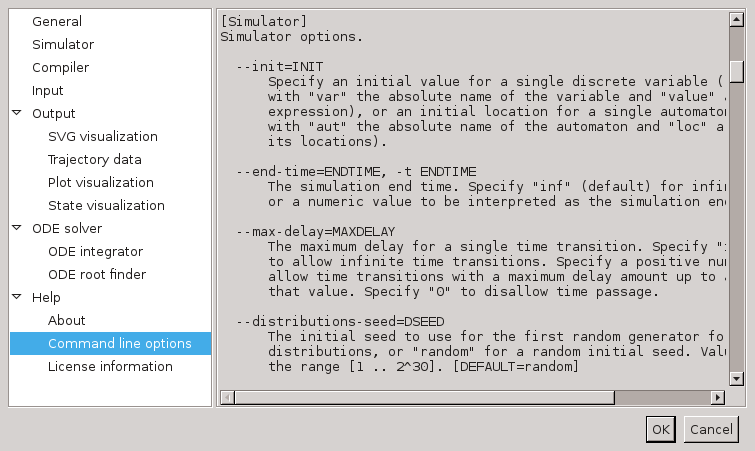
The option dialog shows the same help text as the command line --help and
-h options. In this screenshot, you can see the help text of the
--end-time or -t option. This particular option can also be configured
using the option dialog. It is part of the
Simulator
category:
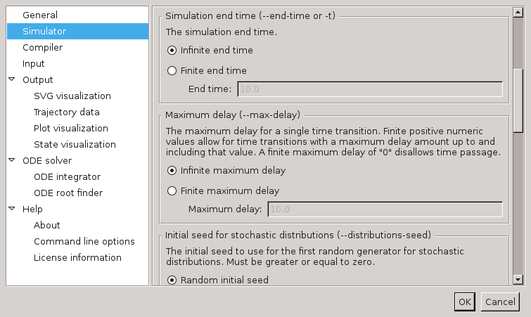
There, it is listed as
Simulator end time
option. After that name,
the command line names of the option (--end-time and -t) are also
listed. This makes it easier to link options in the option dialog with command
line options.
In the example ToolDef scripts so far, all command line arguments are provided as a single string of text. However, it is also possible to provide each command line argument as a separate string. In fact, you may provide as many strings as you like, and each string may contain as many command line arguments as you like. For instance, the following statements each execute the simulator, and all have the same command line arguments, but provided in a different way:
cifsim("some_model.cif -i auto -t 10"); // Single string, all arguments.
cifsim("some_model.cif", "-i auto", "-t 10"); // Multiple strings, multiple arguments each.
cifsim("some_model.cif", "-i", "auto", "-t", "10"); // Multiple strings, one argument each.For simulations, disabling a certain simulation option is a common task. By listing each simulation option on a separate line of the script, disabling or enabling a simulation option becomes as easy as commenting or uncommenting a line of the script. For instance, consider the following script:
from "lib:cif" import *;
cifsim(
"some_model.cif",
"-i auto",
"-t 10",
);The model to simulate, the enabling of the automatic input mode, and the simulation end time, are each specified on a separate line. This makes it very easy to disable the simulation end time:
from "lib:cif" import *;
cifsim(
"some_model.cif",
"-i auto",
// "-t 10",
);To comment a line or multiple selected lines in a ToolDef text editor, use
keyboard shortcut Ctrl+/ or the corresponding toolbar button
( ). For uncommenting, use keyboard shortcut
Ctrl+Shift+/ or the corresponding toolbar button
(
). For uncommenting, use keyboard shortcut
Ctrl+Shift+/ or the corresponding toolbar button
( ).
).
Output redirection and other options
Besides the application specific options that can be configured using the
command line arguments, all tools such as the cifsim tool, have some
additional options. This includes the possibility to write the output of the
tool to a file instead of the console:
from "lib:cif" import *;
cifsim("some_model.cif -i auto -t 10", stdout="output.txt");The stdout parameter of the cifsim tool is used to specify the
filename of the file to which to write the output. A complete list of the
available parameters and their meaning, is available on the
Overview of scriptable tools page.
Overview of scriptable tools
This page provides an overview of the CIF tools that are available in the
cif library that is registered with ToolDef by CIF.
Tools
The following table shows the relation between the names of the ToolDef tools in the library and the tools of the CIF tool set:
| ToolDef tool name | CIF tool |
|---|---|
|
|
|
|
|
|
|
|
|
|
|
|
|
|
|
|
|
|
|
|
|
|
|
|
|
|
|
|
|
|
|
|
|
|
|
|
|
|
|
|
|
|
|
|
|
|
|
|
|
Parameters
For every CIF tool, two ToolDef tool variants are available in the cif
ToolDef library. All the CIF tools in the cif ToolDef library have
the same tool signatures, including the same parameters. Only their names
differ. Below the tool signatures for the two variants are listed, with
toolname instead of the actual tool name (e.g. cifsim):
tool int toolname(
string... args,
string stdin = "-",
string stdout = "-",
string stderr = "-",
bool appendOut = false,
bool appendErr = false,
bool errToOut = false,
bool ignoreNonZeroExitCode = false
)
tool int toolname(
list string args = [],
string stdin = "-",
string stdout = "-",
string stderr = "-",
bool appendOut = false,
bool appendErr = false,
bool errToOut = false,
bool ignoreNonZeroExitCode = false
)The meaning of each of the parameters is as follows:
- args
-
The command line arguments of the application. Each argument string is parsed to zero or more actual arguments. It is possible to use a single string with all arguments (where the arguments themselves are separated by spaces), comma separated strings for each of the arguments (each string has one argument), or a mix of those.
In argument strings, individual arguments are separated by whitespace (spaces, tabs, new lines, etc). The whitespace itself is ignored, and only serves as separation. To include whitespace in an argument, the argument (or a part of it), may be quoted, by putting it between double quotes (
") or single quotes ('). Characters may be escaped by prefixing them with a backslash (\). This is particularly useful for single/double quotes, and escape characters, and can also be used to escape spaces. Escapes work the same inside of quoted parts as they do outside of quoted parts. - stdin
-
Specify whether to have a standard input (stdin) stream and where the input comes from. Use
""to not have a stdin stream, "-" to use the stdin stream of the ToolDef interpreter, or otherwise an absolute or relative local file system path of the file from which to read the standard input. May contain both\and/as path separators - stdout
-
Specify whether to have a standard output (stdout) stream and where to write the standard output. Use
""to not have a stdout stream,"-"to use the stdout stream of the ToolDef interpreter, or otherwise an absolute or relative local file system path of the file to which to write the standard output. May contain both\and/as path separators. - stderr
-
Specify whether to have a standard error (stderr) stream and where to write the standard error output. Use
""to not have a stderr stream,"-"to use the stderr stream of the ToolDef interpreter, or otherwise an absolute or relative local file system path of the file to which to write the standard error output. May contain both\and/as path separators. Is ignored when the standard error stream is redirected to the standard output stream. - appendOut
-
Whether to append to the stdout file (
true) or overwrite it (false). Is ignored when standard output is not written to a file. - appendErr
-
Whether to append to the stderr file (
true) or overwrite it (false). Is ignored if standard error output is not written to a file. Is also ignored when standard error stream is redirected to the standard output stream. - errToOut
-
Whether to redirect the standard error stream to the standard output stream (
true) or use separate streams (false). - ignoreNonZeroExitCode
-
Whether to ignore non-zero exit codes (
true) or consider them as errors (false).
Return value
All the tools return an integer value. This value is the exit code of the
application. A zero (0) exit code means the application terminated without
any errors. A non-zero exit code means the application terminated with an
error.
Implementation
All the tools are internally implemented using the ToolDef app tool.
CIF examples
CIF ships with several examples. To obtain these examples, follow these steps:
-
Start the Eclipse ESCET IDE.
-
Click .
-
Select CIF Examples and click Next.
-
Choose the name of the new project that will be created.
-
Choose a location for the new project, on your hard disk. If you leave the Use default location option enabled, the new project will be created in workspace directory. See the Eclipse ESCET documentation for more information on workspaces.
-
Click Finish to create the new project, and fill it with the examples.
For new releases of CIF, the examples may change. The examples project that you previously created won’t be automatically updated. You can however go through the steps again, and get a second project, with the new examples. The version of the release is included in the suggested project name, allowing multiple example projects for different releases.
Most examples also include a ToolDef script
(.tooldef file) that can be used to perform various tasks, such as
simulation. To execute such a script, right click a .tooldef file an choose
Execute ToolDef. Alternatively, select the file and press
F10.
CIF release notes
The release notes for the releases of CIF and the associated tools, as part of the Eclipse ESCET project, are listed below in reverse chronological order.
See also the Eclipse ESCET toolkit release notes covering those aspects that are common to the various Eclipse ESCET tools.
Version 0.1
The first release of CIF as part of the Eclipse ESCET project. This release is based on the initial contribution by the Eindhoven University of Technology (TU/e).
Most notable changes compared to the last TU/e release:
-
The names of the CIF command line tools and tools available in ToolDef scripts have changed. For more information, check the list of currently available tools.
-
The CIF simulator no longer crashes on code generation.
-
The CIF simulator plot visualizer has been re-implemented using different third party libraries.
Developers
The CIF developers manual is intended only for those who develop or extend the CIF language or tools. It is not intended for end users.
This manual only contains CIF specific information. For general developers information, see the Eclipse ESCET developers manual.
The following information is available for developers:
CIF language modification
For each change to the CIF language, follow these steps:
-
Update
cif.setextsyntax. -
Update
cif.bnfsyntax in documentation. -
Update example models for changed syntax.
-
Update Ecore metamodel. Update Ecore diagram images.
-
Update Ecore genmodel. Remove and re-generate model code.
-
Update generated Java constructors and walker code.
-
Update LaTeX documentation skeleton files.
-
Update LaTeX documentation, including constraints. Generate new PDF.
-
Update example models for changed constraints.
-
Update parser implementation, including AST classes.
-
Update text editor, including keywords and syntax highlighting.
-
Update type checker, including error message enumeration.
-
Update pretty printer, including set of keywords.
-
Update CIF to CIF transformations and other tools.
-
Update CIF documentation, including language reference manual with lexical syntax and grammar.
-
Update CIF syntax highlighting definition for LaTeX.
-
Update CIF syntax highlighting definition for AsciiDoctor.
Legal
The material in this documentation is Copyright (c) 2010, 2021 Contributors to the Eclipse Foundation.
Eclipse ESCET and ESCET are trademarks of the Eclipse Foundation. Eclipse, and the Eclipse Logo are registered trademarks of the Eclipse Foundation. Other names may be trademarks of their respective owners.
License
The Eclipse Foundation makes available all content in this document ("Content"). Unless otherwise indicated below, the Content is provided to you under the terms and conditions of the MIT License. A copy of the MIT License is available at https://opensource.org/licenses/MIT. For purposes of the MIT License, "Software" will mean the Content.
If you did not receive this Content directly from the Eclipse Foundation, the Content is being redistributed by another party ("Redistributor") and different terms and conditions may apply to your use of any object code in the Content. Check the Redistributor’s license that was provided with the Content. If no such license exists, contact the Redistributor. Unless otherwise indicated below, the terms and conditions of the MIT License still apply to any source code in the Content and such source code may be obtained at http://www.eclipse.org.